


13–22 Programming Techniques
File name 33s-English-Manual-040130-Publication(Edition 2).doc Page : 388
Printed Date : 2004/1/30 Size : 13.7 x 21.2 cm
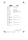
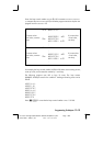
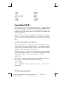
STO(i)
RCL(i)
STO +, –,
×
,
÷
, (i)
RCL +, –,
×
,
÷
, (i)
XEQ(i)
GTO(i)
X<>(i)
INPUT(i)
VIEW(i)
DSE(i)
ISG(i)
SOLVE(i)
∫
FN d(i)
FN=(i)
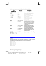
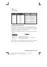
Program Control with (i)
Since the contents of i can change each time a program runs — or even in different
parts of the same program — a program instruction such as
can branch
to a different label at different times. This maintains flexibility by leaving open (until
the program runs) exactly which variable or program label will be needed. (See
the first example below.)
Indirect addressing is very useful for counting and controlling loops. The variable
i
serves as an
index, holding the address of the variable that contains the
loop–control number for the functions DSE and ISG. (See the second example
below.)
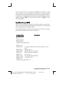
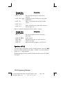
Example: Choosing Subroutines With (i).
The "Curve Fitting" program in chapter 16 uses indirect addressing to determine
which model to use to compute estimated values for
x and y. (Different subroutines
compute
x and y for the different models.) Notice that i is stored and then indirectly
addressed in widely separated parts of the program.
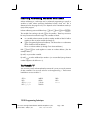
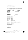
The first four routines (S, L, E, P) of the program specify the curve–fitting model that
will be used and assign a number (1, 2, 3, 4) to each of these models. This number
is then stored during routine Z, the common entry point for all models:
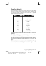
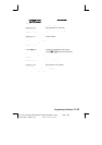
Routine Y uses
i to call the appropriate subroutine (by model) to calculate the x–
and
y–estimates. Line Y0003 calls the subroutine to compute
y
ˆ
:
and line Y0008 calls a different subroutine to compute
x
ˆ
after i has been
increased by 6: