3.8. MODEL REDUCTION 125
3.8.3 Hankel Singular Value Approximation
The function ophank (also cross-licensed from the Model Reduction Module) is used to
perform optimal Hankel norm approximation. Recall from Section 2.6.3 that there is an
astable system achieving the lower bound. The unstable part of this system is returned
as the second argument.
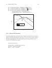
The following applies the Hankel norm approximation technique to the previous
example. The unstable part of the optimal approximation is sysout4u and the astable
system, sysout4 + sysout4u would achieve the lower bound for the approximation
error. The Hankel singular values can also be obtained by this function.
# Optimal Hankel singular value approximation
[sysout4,sysout4u,hsv] = ophank(sys1,{nsr=3})
sysout4g = freq(sysout4,fHz)
hankerr = sys1g - sysout4g
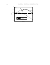
# Compare to the errors from the previous example.
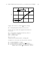
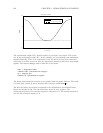
g3 = ctrlplot(sys1g,{logmagplot});
g3 = ctrlplot(sysout4g,g3,{logmagplot,line
style=2});
g3 = ctrlplot(hankerr,g3,{logmagplot,line
style=6});
g3 = ctrlplot(balerr,g3,{logmagplot,line
style=4});
g3 = ctrlplot(residerror,g3,{logmagplot,line
style=5});
g3 = plot(g3,{!grid,legend=["original system";...
"Hankel norm approximation";"error: ophank";...
"error: balmoore";"error: sresidualize"]})?


