4.1. THE HIMAT EXAMPLE 137
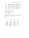
-2.2517e-02 0.0000e+00 2.2517e-02 1.0000
-2.2600e-02 0.0000e+00 2.2600e-02 1.0000
-3.0000e-02 0.0000e+00 3.0000e-02 1.0000
-3.0000e-02 0.0000e+00 3.0000e-02 1.0000
-2.9369e+00 0.0000e+00 2.9369e+00 1.0000
-2.9974e+00 0.0000e+00 2.9974e+00 1.0000
-4.8310e+00 0.0000e+00 4.8310e+00 1.0000
-6.5876e+00 0.0000e+00 6.5876e+00 1.0000
-5.8350e+01 -5.6049e+01 8.0909e+01 0.7212
-5.8350e+01 5.6049e+01 8.0909e+01 0.7212
-8.8792e+01 -4.2881e+01 9.8604e+01 0.9005
-8.8792e+01 4.2881e+01 9.8604e+01 0.9005
-9.9778e+01 0.0000e+00 9.9778e+01 1.0000
-7.4258e+03 0.0000e+00 7.4258e+03 1.0000
-1.0000e+04 0.0000e+00 1.0000e+04 1.0000
-1.0000e+04 0.0000e+00 1.0000e+04 1.0000
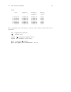
Zeros:
ans (a scalar) = 0
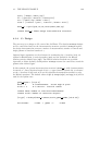
Now calculate a closed loop frequency response. This results in a 4x4 pdm: g1g
g1g=freq(g1,om2)
comment g1g "frequency response of g1"
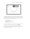
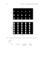
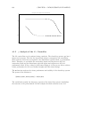
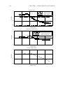
The singular values of the closed loop system are calculated. The maximum of the
singular values over frequency is also calculated and compared to γ.Asγis a
guaranteed upper bound on the infinity norm, this value should be less.
g1gs = svd(g1g)
comment g1gs "closed loop singular value: iteration 1"
gph3 = ctrlplot(g1gs,{log});
gph3 = plot(gph3,{!grid,...
title="Singular value plot of the closed loop"})?


