150 CHAPTER 4. DEMONSTRATION EXAMPLES
The loopshaping design gives a decoupled response. Both the H
∞
and µ designs trade
decoupling for speed of response and, as we shall see, robustness with respect to
perturbations.
The simulation is repeated with a perturbation of size 0.1. Note that this is only 10% of
the size perturbation that we were analyzing and designing for in the above.
delta = [.1,0;0,-0.1]
comment delta "example perturbation"
gsim
mu pert = starp(delta,gsim mu)
gsim
hinf pert = starp(delta,gsim hinf)
gsim
lp pert = starp(delta,gsim lp)
comment gsim
mu pert "perturbed closed loop sys: mu ctrl"
comment gsim
hinf pert "perturbed closed loop sys: hinf ctrl"
comment gsim
lp pert "perturbed closed loop sys: klp ctrl"
y
mu pert = gsim mu pert*u
y
hinf pert = gsim hinf pert*u
y
lp pert = gsim lp pert*u
comment y
mu pert "perturbed response: mu ctrl"
comment y
hinf pert "perturbed response: hinf ctrl"
comment y
lp pert "perturbed response: klp ctrl"
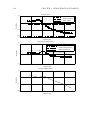
The loop shaping controller performs poorly on the perturbed system. Again the time
response of each system is plotted.
gph8 = plot(y
mu pert,{rows=3,row=1,grid,...
title="Kmu step dist. response (perturbed)",...
x
lab="time",y max=1.5,y min=-1});
gph8 = plot(y
hinf pert,gph8,{row=2,grid,...
title="Kinf step dist. response (perturbed)",...
x
lab="time",y max=1.5,y min=-1});
gph8 = plot(y
lp pert,gph8,{row=3,grid,...
title="Klp step dist. response: (perturbed)",...
x
lab="time",y max=1.5,y min=-1})?


