8 CHAPTER 2. OVERVIEW OF THE UNDERLYING THEORY
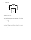
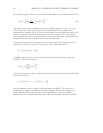
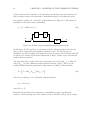
is interpreted to mean that the signal y is the sum of the response of system P
21
to
input signal v and system P
22
to input signal u. In general, we will not be specific about
the representation of the system P. If we do need to be more specific about P,then
P(s) is the Laplace representation and p(t) is the impulse response.
Note that Figure 2.1 is drawn from right to left. We use this form of diagram because it
more closely represents the order in which the systems are written in the corresponding
mathematical equations. We will later see that the particular block diagram shown in
Figure 2.1 is used as a generic description of a robust control system.
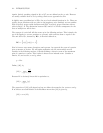
In the case where we are considering a state-space representation, the following notation
is also used. Given P(s), with state-space representation,
sx(s)=Ax(s)+Bu(s)
y(s)=Cx(s)+Du(s),
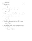
we associate this description with the notation,
P(s)=
A
B
C D
.
The motivation for this notation comes from the example presented in Section 2.2.4. We
will also use this notation to for state-space representation of discrete time systems
(where s in the above is replaced by z). The usage will be clear from the context of the
discussion.
2.1.2 An Introduction to Norms
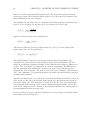
A norm is simply a measure of the size of a vector, matrix, signal, or system. We will
define and concentrate on particular norms for each of these entities. This gives us a
formal way of assessing whether or not the size of a signal is large or small enough. It
allows us to quantify the performance of a system in terms of the size of the input and
output signals.
Unless stated otherwise, when talking of the size of a vector, we will be using the


