4.2. A SIMPLE FLEXIBLE STRUCTURE EXAMPLE 179
Now we consider the closed-loop nominal response with Khinf and Kmu. The closed-loop
system happens to have a large number of high frequency poles which do not contribute
significantly to the response. They have the effect of forcing a very fine time
discretization in the simulation, resulting in a long calculation time. We remove all poles
of frequency greater than 100 rad/sec. by residualization. This is not intended as a
general procedure — in some situations the high frequency behavior will be significant.
nomclp = starp(deltazero,Pnom)
nomclphinf = starp(nomclp,Khinf)
nomclpmu = starp(nomclp,Kmu)
fmax = 100;
nlfpoles = sum(abs(poles(nomclphinf))<fmax)
str = "Residualizing closed loop system to " + ...
string(nlfpoles)+" states"
display(str)
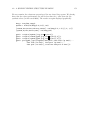
Residualizing closed loop system to 6 states
nsysclphinf = modalstate(nomclphinf)
nsysclphinf = sresidualize(nsysclphinf,nlfpoles)
nlfpoles = sum(abs(poles(nomclpmu))<fmax)
nsysclpmu = modalstate(nomclpmu)
nsysclpmu = sresidualize(nsysclpmu,nlfpoles)
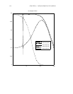
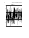
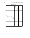
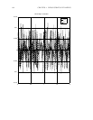
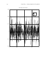
The closed-loop responses are calculated and plotted.
yclphinf = nsysclphinf*u
yclpmu = nsysclpmu*u
gph10 = ctrlplot(yclphinf(1,1));
gph10 = ctrlplot(yclpmu(1,1),gph10);
gph10 = plot(gph10,{legend=["Khinf";"Kmu"],...
title="closed loop beam length",...
y
lab="micrometers"})?


