4.2. A SIMPLE FLEXIBLE STRUCTURE EXAMPLE 185
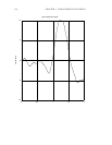
Note that Kmu achieves better performance at the expense of greater actuator effort.
We will now repeat this simulation for a perturbed system. A bad ∆ is chosen and
scaled to have norm 0.5. This is obtained from destabilizing ∆ calculated for the µ lower
bound. An all-pass system is fitted to ∆ at one frequency to create a real-rational
perturbation. The frequency selected is that where µ is at its maximum. In this case we
choose the ∆ that comes from the robust stability µ test. This gives the perturbation
which comes closest to destabilizing the closed loop system. Using ∆ from the robust
performance test would allow us to create a perturbation which minimizes the robust
performance of the closed loop system.
Here we use the worst-case ∆ for Kmu. This is almost certainly not the worst-case ∆ for
Khinf. Again, the closed loop systems are residualized prior to calculating the responses.
deltabad = mkpert(Deltars,blk(1:2,1:2),rsbnds,{pnorm=0.5})
badclp = starp(deltabad,Pnom)
badclphinf = starp(badclp,Khinf)
badclpmu = starp(badclp,Kmu)
nlfpoles = sum(abs(poles(badclphinf))<fmax)
str = "Residualizing closed loop system to "+...
string(nlfpoles)+" states"
display(str)
Residualizing closed loop system to 6 states
nbclphinf = modalstate(badclphinf)
nbclphinf = sresidualize(nbclphinf,nlfpoles)
nlfpoles = sum(abs(poles(badclpmu))<fmax)
nbclpmu = modalstate(badclpmu)
nbclpmu = sresidualize(nbclpmu,nlfpoles)
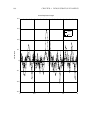
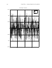
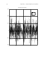
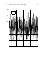
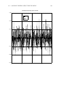
The responses are calculated and plotted.
ybclphinf = nbclphinf*u
ybclpmu = nbclpmu*u
gph13 = ctrlplot(ybclphinf(1,1));


