2.2. MODELING UNCERTAIN SYSTEMS 13
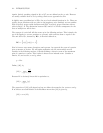
The set of all systems with bounded ∞-norm is denoted by L
∞
. We can again split this
into stable and unstable parts. H
∞
denotes the stable part; those systems with |P(s)|
finite for all Re(s)> 0. This is where the name “H
∞
control theory” originates, and we
often call this norm the H
∞
-norm. Again we can restrict ourselves to real rational
functions, so RL
∞
is the set of proper transfer functions with no poles on the ω axis.
Similary, RH
∞
is the set of proper, stable transfer functions.
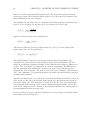
Again, we are free to choose a spatial norm for the input and output signals u(s)and
y(s). In keeping with our above choices we will choose the Euclidean norm. So if P(s)is
a MIMO system, then,
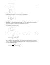
P(s)
∞
=sup
ω
σ
max
[P(ω)].
There is another choice of system norm that will arise in the following sections. This is
the H
2
-norm for systems, defined as,
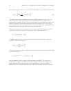
P(s)
2
=
1
2π
∞
−∞
Trace[P(ω)
∗
P(ω)]dω
1/2
,
where P(ω)
∗
denotes the conjugate transpose of P(ω) and the trace of a matrix is the
sum of its diagonal elements. This norm will come up when we are considering linear
quadratic Gaussian (LQG) problems.
2.2 Modeling Uncertain Systems
2.2.1 Perturbation Models for Robust Control
A simple example will be used to illustrate the idea of a perturbation model. We are
interested in describing a system by a set of models, rather than just a nominal model.
Our uncertainty about the physical system will be represented in an unknown
component of the model. This unknown component is a perturbation, ∆, about which
we make as few assumptions as possible; maximum size, linearity, time-invariance, etc..
Every different perturbation, ∆, gives a slightly different system model. The complete


