2.2. MODELING UNCERTAIN SYSTEMS 15
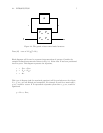
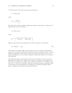
as specifying a maximum percentage error between P
nom
and every other element of P.
The system P
nom
(s) is the element of P that comes from ∆ = 0 and is called the
nominal system. In otherwords, for ∆ = 0, the input-output relationship is
y(s)=P
nom
(s)u(s). As ∆ deviates from zero (but remains bounded in size), the
nominal system is multiplied by (I +∆W
m
(s)). W
m
(s) is a frequency weighting function
which allows us the specify the maximum effect of the perturbation for each frequency.
Including W
m
(s) allows us to model P with ∆ being bounded by one. Any
normalization of ∆ is simply included in W
m
(s).
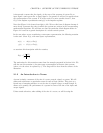
We often assume that ∆ is also linear and time-invariant. This means that ∆(ω)is
simply an unknown, complex valued matrix at each frequency, ω.If∆
∞
≤1, then, at
each frequency, σ
max
(∆(ω)) ≤ 1. Section 2.2.3 gives a further discussion on the pros
and cons of considering ∆ to be linear, time-invariant.
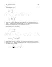
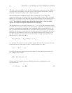
Now consider an example of this approach from a Nyquist point of view. A simple first
order SISO system with multiplicative output uncertainty is modeled as
y(s)=
(I+W
m
(s)∆)P
nom
(s)
u(s),
where
P
nom
(s)=
1+0.05s
1+s
and W
m
(s)=
0.1+0.2s
1+0.05s
.
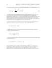
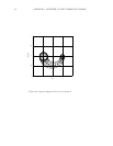
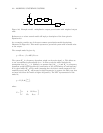
Figure 2.3 illustrates the set of systems generated by a linear time-invariant ∆,
∆
∞
≤ 1.
At each frequency, ω, the transfer function of every element of P, lies within a circle,
centered at P
nom
(ω), of radius |P
nom
(ω)W
m
(ω)|. Note that for certain frequencies the
disks enclose the origin. This allows us to consider perturbed systems that are
non-minimum phase even though the nominal system is not.
It is worth pointing out that P is still a model; in this case a set of regions in the
Nyquist plane. This is model set is now able to describe a larger set of system behaviors
than a single nominal model. There is still an inevitable mismatch between any model
(robust control model set or otherwise) and the behaviors of a physical system.


