18 CHAPTER 2. OVERVIEW OF THE UNDERLYING THEORY
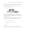
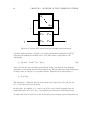
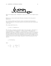
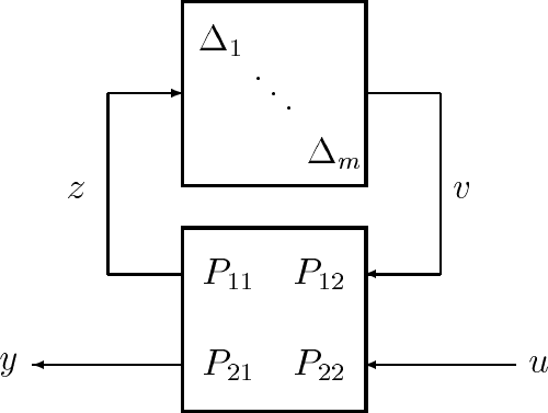
Figure 2.5: Generic LFT model structure including perturbations,∆
A generic model structure, referred to as a linear fractional transformation (LFT),
overcomes the difficulties outlined above. The LFT model is equivalent to the
relationship,
y =
P
21
∆(I − P
11
∆)
−1
P
12
+ P
22
u, (2.6)
where the ∆ is the norm bounded perturbation. Figure 2.5 shows a block diagram
equivalent to the system described by Equation 2.6. Because this form of interconnection
is widely used, we will give it a specific notation. Equation 2.6 is abbreviated to,
y = F
u
(P,∆)u.
The subscript, u, indicates that the ∆ is closed in the upper loop. We will also use
F
l
(.,.) when the lower loop is closed.
In this figure, the signals, u, y, z and v can all be vector valued, meaning that the
partitioned parts of P,(P
11
, etc.) can themselves be matrices of transfer functions.
To make this clear we will look at the perturbed system example, given in Equation 2.4,


