22 CHAPTER 2. OVERVIEW OF THE UNDERLYING THEORY
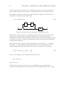
Robust control models are therefore set descriptions. In the analysis of such models it is
also assumed that the unknown inputs belong to some bounded set. Several choices of
set for the unknown signals can be made, leading to different mathematical problems for
the analysis. Unfortunately not all of them are tractable. The following section discusses
the assumptions typically applied to the robust control models.
2.2.3 Assumptions on P, ∆, and the unknown signals
It will be assumed that the elements of P are either real-rational transfer function
matrices or complex valued matrices. The second case arises in the frequency by
frequency analysis of systems.
In modeling a system, P
22
defines the nominal model. Input/output effects not
described by the nominal model can be attributed to either unknown signals which are
components of the model input (w in the previous example), or the perturbation ∆.
Unmodeled effects which can destabilize a system should be accounted for in ∆. The ∆
can loosely be considered as accounting for the following. This list is by no means
definitive and is only included to illustrate some of the physical effects better suited to
description with ∆.
• Unmodeled dynamics. Certain dynamics may be difficult to identify and there
comes a point when further identification does not yield significant design
performance improvement.
• Known dynamics which have been bounded and included in ∆ to simplify the
model. As the controller complexity depends on the order of the nominal model a
designer may not wish to explicitly include all of the known dynamics.
• Parameter variations in a differential equation model. For example linearization
constants which can vary over operating ranges.
• Nonlinear or inconsistent effects. At some point a linear model will no longer
account for the residual differences between the behaviors of the model and the
physical system.
Several assumptions on ∆ are possible. In the most general case ∆ is a bounded
operator. Alternatively ∆ can be considered as a linear time varying multiplier. This
assumption can be used to capture nonlinear effects which shift energy between
frequencies. Analysis and synthesis are possible with this assumption; Doyle and


