30 CHAPTER 2. OVERVIEW OF THE UNDERLYING THEORY
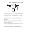
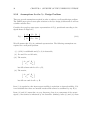
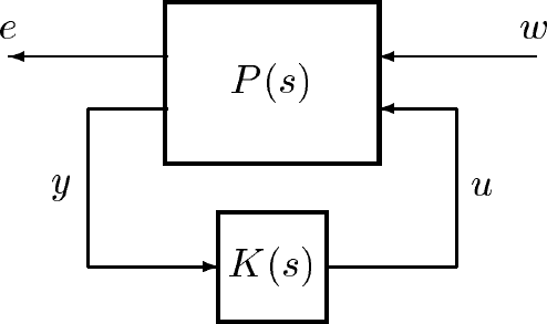
Figure 2.7: LFT configuration for controller synthesis, G(s)=F
l
[P(s),K(s)]
Note that the interconnection structure, P(s), given here, differs from that discussed in
the previous section. Here we set up P(s) so that the input, w, is the unknown signals
entering our system. Typical examples would be sensor noise, plant disturbances or
tracking commands. The output, e, represent signals that we would like to make small.
In an engineering application these could include actuator signals and tracking errors.
The signal y is the measurement available to the controller, K(s). In any realistic
problem, some weighted component of w would be added to y to model sensor noise.
The output of the controller, u, is our actuation input to the system. Again, a
reasonable engineering problem would include a weighted u signal as a component of the
penalty output, e.
The interconnection structure, P(s), also contains any frequency weightings on the
signals e and w. Weightings on components of e are used to determine the relative
importance of the various error signals. Weight functions on w indicate the relative
expected size of the unknown inputs.
Xµ provides functions to calculate the controllers minimizing either the H
2
or H
∞
norm
of G(s). We will cover both of these approaches in the context of the design problem
illustrated in Figure 2.7.
Note that neither of these design approaches takes advantage of any information about
structured perturbations occuring within the model. The following discussion can be
considered as applying to a nominal design problem. Section 2.5 uses D-K iteration to


