


Example:
4.123.586.4 = 21.1496
4.123.587.1 = 7.6496
[ON/AC] [4] [•] [1] [2] []
[3] [•] [5] [8] [] [6] [•] [4] [=]
[3]
[3] [3] [3] [3]
[] [7] [•] [1]
[=]
The replay function is not cleared even when [ON/AC] is
pressed or when power is turned OFF, so contents can be
recalled even after [ON/AC] is pressed.
Replay function is cleared when mode or operation is
switched.
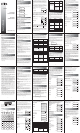
Error Position Display Function
When an ERROR message appears during operation
execution, the error can be cleared by pressing the
[ON/AC] key, and the values or formula can be re-entered
from the beginning. However, by pressing the [3] or [4]
key, the ERROR message is cancelled and the cursor moves
to the point where the error was generated.
Example: 1402.3 is input by mistake
[ON/AC] [1] [4] [] [0] []
[2] [.] [3] [=]
[3] (or [4] )
Correct the input by pressing
[3] [SHIFT] [INS] [1]
[=]
Scientific Function
Trigonometric functions and inverse trigonometric
functions
• Be sure to set the unit of angular measurement before
performing trigonometric function and inverse
trigonometric function calculations.
• The unit of angular measurement (degrees, radians,
grads) is selected in sub-menu.
• Once a unit of angular measurement is set, it remains in
effect until a new unit is set. Settings are not cleared
when power is switched OFF.
Performing Hyperbolic and Inverse Hyperbolic Functions
Logarithmic and Exponential Functions
Coordinate Transformation
• This scientific calculator lets you convert between
rectangular coordinates and polar coordinates, i.e., P(x, y)
↔ P(r, )
• Calculation results are stored in variable memory E and
variable memory F. Contents of variable memory E are
displayed initially. To display contents of memory F,
press [RCL] [F].
• With polar coordinates, can be calculated within a
range of –180
º
< ≤180
º
.
(Calculated range is the same with radians or grads.)
Permutation and Combination
Total number of permutations nPr = n!/(nr)!
Total number of combinations nCr = n!/(r!(nr)!)
Other Functions (√ , x
2
, x
–1
, x!,
3
√, Ran#)
Fractions
Fractions are input and displayed in the order of integer,
numerator and denominator. Values are automatically
displayed in decimal format whenever the total number of
digits of a fractional value (interger + numerator +
denominator + separator marks) exceeds 10.
Degree, Radian, Gradient Interconversion
Degree, radian and gradient can be converted to each
other with the use of [SHIFT][DRG>]. Once [SHIFT]
[DRG>] have been keyed in, the "DRG" selection menu
will be shown as follows.
Degrees, Minutes, Seconds Calculations
You can perform sexagesimal calculations using degrees
(hours), minutes and seconds. And convert between
sexagesimal and decimal values.
Statistical Calculations
This unit can be used to make statistical calculations
including standard deviation in the "SD" mode, and
regression calculation in the "REG" mode.
Standard Deviation
In the "SD" mode, calculations including 2 types of
standard deviation formulas, mean, number of data, sum
of data, and sum of square can be performed.
Data input
1. Press [MODE] [2] to specify SD mode.
2. Press [SHIFT] [Scl] [=] to clear the statistical memories.
3. Input data, pressing [DT] key (= [M+]) each time a new
piece of data is entered.
Example Data: 10, 20, 30
Key operation: 10 [DT] 20 [DT] 30 [DT]
• When multiples of the same data are input, two different
entry methods are possible.
Example 1 Data: 10, 20, 20, 30
Key operation: 10 [DT] 20 [DT] [DT] 30 [DT]
The previously entered data is entered again each time
the DT is pressed without entering data (in this case 20
is re-entered).
Example 2 Data: 10, 20, 20, 20, 20, 20, 20, 30
Key operation: 10 [DT] 20 [SHIFT] [;] 6 [DT] 30 [DT]
By pressing [SHIFT] and then entering a semicolon
followed by value that represents the number of items the
data is repeated (6, in this case) and the [DT] key, the
multiple data entries (for 20, in this case) are made
automatically.
Deleting input data
There are various ways to delete value data, depending on
how and where it was entered.
Example 1 40 [DT] 20 [DT] 30 [DT] 50 [DT]
To delete 50, press [SHIFT] [CL].
Example 2 40 [DT] 20 [DT] 30 [DT] 50 [DT]
To delete 20, press 20 [SHIFT] [CL].
Example 3 30 [DT] 50 [DT] 120 [SHIFT] [;]
To delete 120 [SHIFT] [;] , press [ON/AC].
Example 4 30 [DT] 50 [DT] 120 [SHIFT] [;] 31
To delete 120 [SHIFT] [;] 31, press [AC].
Example 5 30 [DT] 50 [DT] 120 [SHIFT] [;] 31 [DT]
To delete 120 [SHIFT] [;] 31 [DT], press [SHIFT] [CL].
Example 6
50 [DT] 120 [SHIFT] [;] 31 [DT] 40 [DT] 30 [DT]
To delete 120 [SHIFT] [;] 31
[DT]
, press 120 [SHIFT] [;] 31
[SHIFT] [CL].
Example 7 [√] 10
[DT]
[√] 20
[DT]
[√] 30
[DT]
To delete [√] 20
[DT]
, press [√] 20 [=] [Ans] [SHIFT] [CL].
Example 8 [√] 10
[DT]
[√] 20
[DT]
[√] 30
[DT]
To delete [√] 20
[DT]
, press [√] 20 [SHIFT] [;] [(–)] 1
[DT]
.
Performing calculations
The following procedures are used to perform the various
standard deviation calculations.
Standard deviation and mean calculations are performed
as shown below:
Population standard deviation σn = √(∑(x
i
x)
2
/n)
where i = 1 to n
Sample standard deviation σn–1 = √(∑(x
i
x)
2
/(n-1))
where i = 1 to n
Mean x = (∑x)/n
Regression Calculation
In the REG mode, calculations including linear regression,
logarithmic regression, exponential regression, power
regression, inverse regression and quadratic regression
can be performed.
Press [MODE] [3] to enter the "REG" mode:
and then select one of the following regression types:-
Lin: linear regression
Log: logarithmic regression
Exp: exponential regression
press [4] for the other three regression types:-
Pwr: power regression
Inv: inverse regression
Quad: quadratic regression
Linear regression
Linear regression calculations are carried out using the
following formula:
y = A + Bx.
Data input
Press [MODE] [3] [1] to specify linear regression under
the "REG" mode.
Press [Shift] [Scl] [=] to clear the statistical memories.
Input data in the following format: <x data> [,] <y data>
[DT]
• When multiples of the same data are input, two different
entry methods are possible:
Example 1 Data: 10/20, 20/30, 20/30, 40/50
Key operation: 10 [,] 20 [DT]
20 [,] 30 [DT] [DT]
40 [,] 50 [DT]
The previously entered data is entered again each time
the [DT] key is pressed (in this case 20/30 is re-entered).
Example 2 Data: 10/20, 20/30, 20/30, 20/30, 20/30, 20/30,
40/50
Key operation: 10 [,] 20 [DT]
20 [,] 30 [SHIFT] [;] 5 [DT]
40 [,] 50 [DT]
By pressing [SHIFT] and then entering a semicolon
followed by a value that represents the number of times
the data is repeated (5, in this case) and the [DT] key, the
multiple data entries (for 20/30, in this case) are made
automatically.
Deleting input data
There are various ways to delete value data, depending on
how and where it was entered.
Example 1 10 [,] 40 [DT]
20 [,] 20 [DT]
30 [,] 30 [DT]
40 [,] 50
To delete 40 [,] 50, press [ON/AC]
Example 2 10 [,] 40 [DT]
20 [,] 20 [DT]
30 [,] 30 [DT]
40 [,] 50 [DT]
To delete 40 [,] 50 [DT], press [SHIFT][CL]
Example 3
To delete 20 [,] 20 [DT], press 20 [,] 20 [SHIFT][CL]
Example 4 [√] 10 [,] 40 [DT]
[√] 40 [,] 50 [DT]
To delete[√]10[,]40[DT],
press [√]10[=][Ans][,]40[SHIFT][CL]
Key Operations to recall regression calculation results
Performing calculations
The following procedures are used to perform the various
linear regression calculations.
The regression formula is y = A + Bx. The constant term of
regression A, regression coefficient B, correlation r,
estimated value of x, and estimated value of y are
calculated as shown below:
A = ( ∑y∑x )/n
B = ( n∑xy∑x∑y ) / ( n∑x
2
(∑x )
2
)
r = ( n∑xy∑x∑y ) / √ (( n∑x
2
(∑x )
2
)( n∑y
2
(∑y )
2
))
y = A + Bx
x = ( yA) / B
Logarithmic regression
Logarithmic regression calculations are carried out using
the following formula:
y = A + B•lnx
Data input
Press [MODE] [3] [2] to specify logarithmic regression
under "REG" mode.
Press [SHIFT] [Scl] [=] to clear the statistical memories.
Input data in the following format: <x data>, <y data>
[DT]
• To make multiple entries of the same data, follow
procedures described for linear regression.
Deleting input data
To delete input data, follow the procedures described for
linear regression.
Performing calculations
The logarithmic regression formula y = A + B•lnx. As x is
input, In(x) will be stored instead of x itself. Hence, we can
treat the logarithmic regression formula same as the
linear regression formula. Therefore, the formulas for
constant term A, regression coefficient B and correlation
coefficient r are identical for logarithmic and linear
regression.
A number of logarithmic regression calculation results
differ from those produced by linear regression. Note the
following:
Exponential regression
Exponential regression calculations are carried out using
the following formula:
y = A•e
B•x
(ln y = ln A +Bx)
Data input
Press [MODE] [3] [3] to specify exponential regression
under the "REG" mode.
Press [SHIFT] [Scl] [=] to clear the statistical memories.
Input data in the following format: <x data>,<y data> [DT]
• To make multiple entries of the same data, follow
procedures described for linear regression.
Deleting input data
To delete input data, follow the procedures described for
linear regression.
Performing calculations
If we assume that lny = y and lnA = a', the exponential
regression formula y = A•e
B•x
(ln y = ln A +Bx) becomes
the linear regression formula y =a' + bx if we store In(y)
instead of y itself. Therefore, the formulas for constant
term A, regression coefficient B and correlation coefficient
r are identical for exponential and linear regression.
A number of exponential regression calculation results
differ from those produced by linear regression. Note the
following:
Power regression
Power regression calculations are carried out using the
following formula:
y = A•x
B
(lny = lnA + Blnx)
Data input
Press [MODE] [3] [4] [1] to specify "power regression".
Press [SHIFT] [Scl] [=] to clear the statistical memories.
Input data in the following format: <x data>,<y data> [DT]
• To make multiple entries of the same data, follow
procedures described for linear regression.
Deleting input data
To delete input data, follow the procedures described for
linear regression
Performing calculations
If we assume that lny = y, lnA =a' and ln x = x, the power
regression formula y = A•x
B
(lny = lnA + Blnx) becomes
the linear regression formula y = a' + bx if we store In(x)
and In(y) instead of x and y themselves. Therefore, the
formulas for constant term A, regression coefficient B and
correlation coefficient r are identical the power and linear
regression.
A number of power regression calculation results differ
from those produced by linear regression. Note the
following:
Inverse regression
Power regression calculations are carried out using the
following formula:
y = A + ( B/x )
Data input
Press [MODE] [3] [4] [2] to specify "inverse regression".
Press [SHIFT] [Scl] [=] to clear the statistical memories.
Input data in the following format: <x data>,<y data> [DT]
• To make multiple entries of the same data, follow
procedures described for linear regression.
Deleting input data
To delete input data, follow the procedures described for
linear regression
Performing calculations
If 1/x is stored instead of x itself, the inverse regression
formula y = A + ( B/x ) becomes the linear regression
formula y = a + bx. Therefore, the formulas for constant
term A, regression coefficient B and correlation coefficient
r are identical the power and linear regression.
A number of inverse regression calculation results differ
from those produced by linear regression. Note the
following:
Quadratic Regression
Quadratic regression calculations are carried out using the
following formula:
y = A + Bx + Cx
2
Data input
Press [MODE] [3] [4] [3] to specify quadratic regression
under the "REG" mode.
Press [SHIFT] [Scl] [=] to clear the statistical memories.
Input data in this format: <x data>,<y data> [DT]
• To make multiple entries of the same data, follow
procedures described for linear regression.
Deleting input data
To delete input data, follow the procedures described for
linear regression.
Performing calculations
The following procedures are used to perform the various
linear regression calculations.
The regression formula is y = A + Bx + Cx
2
where A, B, C are
regression coefficients.
C = [(n∑x
2
(∑x)
2
) (n∑x
2
y∑x
2
∑y )(n∑x
3
∑x
2
∑x) (n∑xy
∑x∑y)][(n∑x
2
(∑x)
2
) (n∑x
4
(∑x
2
)
2
)(n∑x
3
∑x
2
∑x)
2
]
B = [
n∑xy∑x∑y
C (
n∑x
3
∑x
2
∑x
)]
(
n∑x
2
(
∑x
)
2
)
A = (
∑y
B
∑x
C
∑x
2
) / n
To read the value of
∑x
3
,
∑x
4
or
∑x
2
y
, you can recall
memory [RCL] M, Y and X respectively.
Replacing the Battery
Dim figures on the display of the calculator indicate that
battery power is low. Continued use of the calculator
when the battery is low can result in improper operation.
Replace the battery as soon as possible when display
figures become dim.
To replace the battery:-
• Remove the screws that hold the back cover in place and
then remove the back cover,
• Remove the old battery,
• Wipe off the side of the new battery with a dry, soft cloth.
Load it into the unit with the positive(+) side facing up.
• Replace the battery cover and secure it in place with the
screws.
• Press [ON/AC] to turn power on.
Auto Power Off
Calculator power automatically turns off if you do not
perform any operation for about six minutes. When this
happens, press [ON/AC] to turn power back on.
Specifications
Power supply: AG13 x 2 batteries
Operating temperature: 0
º
~ 40
º
C (32
º
F ~ 104
º
F)
– 20 – – 24 – – 28 – – 32 – – 36 –
– 21 – – 25 – – 29 – – 33 – – 37 –
– 22 –
– 26 – – 30 – – 34 – – 38 –
– 23 – – 27 – – 31 – – 35 –
Display
Example Operation (Lower)
sin 63
º
52'41"
= 0.897859012
cos (π/3 rad) = 0.5
tan (–35 grad)
= –0.612800788
2sin45
º
cos65
º
= 0.597672477
sin
–1
0.5 = 30
cos
–1
(√2/2)
= 0.785398163 rad
= π/4 rad
tan
–1
0.741
= 36.53844577
º
= 36
º
32' 18.4"
If the total number of digits for degrees/minutes/seconds exceed
11 digits, the higher order values are given display priority, and
any lower-order values are not displayed. However, the entire
value is stored within the unit as a decimal value.
2.5
(
sin
–1
0.8
cos
–1
0.9)
= 68
º
13'13.53"
[
MODE
][
MODE
][1]("DEG" selected)
[sin] 63 [
º
' "] 52 [
º
' "]
41 [
º
' "][=]
[
MODE
][
MODE
][2]("RAD" selected)
[cos][(] [
SHIFT
][π][]3
[)] [=]
[
MODE
][
MODE
][3]
("GRA" selected)
[tan] [(–)] 35 [=]
[
MODE
][
MODE
][1]("DEG")
2[sin] 45 [cos] 65 [=]
[
SHIFT
][sin
–1
] 0.5 [=]
[
MODE
][
MODE
][2]("RAD")
[
SHIFT
][cos
–1
][(][√]2 []2
[)][=]
[][
SHIFT
][π][=]
[
MODE
][
MODE
][1]("DEG")
[
SHIFT
][tan
–1
]0.741[=]
[
SHIFT
] [←º' "]
2.5[] [(] [
SHIFT
] [sin
–1
]0.8
[] [
SHIFT
] [cos
–1
] 0.9 [)]
[=] [
SHIFT
] [←º' "]
0.897859012
0.5
–0.612800788
0.597672477
30.
0.785398163
0.25
36.53844576
36
º
32
º
18.4
º
68
º
13
º
13.53
º
4.12x3.58+6.
21.1496
D
4.12x3.58–7.
7.6496
D
Ma ERROR
12x3.58+6.4
_
21.1496
D
12x3.58–7.1
_
21.1496
D
14÷10x2.3
0.
D
14÷10x2.3
3.22
D
Display
Example Operation (Lower)
log1.23
= 8.990511110
–2
In90 = 4.49980967
log456In456
= 0.434294481
10
1.23
= 16.98243652
e
4.5
= 90.0171313
10
4
• e
–4
1.2 • 10
2.3
= 422.5878667
(–3)
4
= 81
–3
4
= –81
5.6
2.3
= 52.58143837
7
√123 = 1.988647795
(7823)
–12
= 1.30511182910
–21
23
3
√644 = 10
23.4
(5+6.7)
= 3306232
[log] 1.23 [=]
[In] 90 [=]
[log]456[In]456 [=]
[
SHIFT
][10
x
] 1.23 [=]
[
SHIFT
][e
x
]4.5[=]
[
SHIFT
][10
x
]4[][
SHIFT
][e
x
]
[(–)]4[]1.2[][
SHIFT
][10
x
]
2.3[=]
[(][(–)] 3 [)] [x
y
] 4 [=]
[(–)] 3 [x
y
] 4 [=]
5.6 [x
y
] 2.3 [=]
7 [
SHIFT
][
x
√] 123 [=]
[(]78[]23[)][x
y
][(–)]12[=]
2[]3[]3[
SHIFT
][
x
√]64
[]4[=]
2[]3.4[x
y
][(]5[]6.7[)][=]
0.089905111
4.49980967
0.434294481
16.98243652
90.0171313
422.5878667
81.
–81.
52.58143837
1.988647795
1.305111829
–21
10.
3306232.001
Display
Example Operation (Lower)
sinh3.6= 18.28545536
cosh1.23 = 1.856761057
tanh2.5= 0.986614298
cosh1.5sinh1.5
= 0.22313016
sinh
–1
30 = 4.094622224
cosh
–1
(20/15)
= 0.795365461
x = (tanh
–1
0.88) / 4
= 0.343941914
sinh
–1
2cosh
–1
1.5
= 1.389388923
sinh
–1
(2/3)tanh
–1
(4/5)
= 1.723757406
[hyp][sin] 3.6 [=]
[hyp][cos] 1.23 [=]
[hyp][tan] 2.5 [=]
[hyp][cos] 1.5 [][hyp]
[sin] 1.5 [=]
[hyp][
SHIFT
][sin
–1
] 30 [=]
[hyp][
SHIFT
][cos
–1
][(] 20
[] 15 [)][=]
[hyp][
SHIFT
][tan
–1
]0.88
[]4[=]
[hyp][
SHIFT
][sin
–1
]2[]
[hyp][
SHIFT
][cos
–1
]1.5[=]
[hyp][
SHIFT
][sin
–1
][(]2[]
3[)][][hyp][
SHIFT
][tan
–1
]
[(]4[]5[)][=]
18.28545536
1.856761057
0.986614298
0.22313016
4.094622224
0.795365461
0.343941914
1.389388923
1.723757406
Display
Example Operation (Lower)
x=14 and y=20.7, what
are r and
º
?
x=7.5 and y=–10, what
are r and rad?
r=25 and = 56
º
, what
are x and y?
r=4.5 and =2π/3 rad,
what are x and y?
[
MODE
][
MODE
][1]("DEG" selected)
[Pol(]14 [
,
]20.7[)][=]
[RCL][F]
[
SHIFT
][←º' "]
[
MODE
][
MODE
][2]("RAD" selected)
[
Pol(
]
7.5
[
,
][(–)]
10
[)][=]
[RCL][F]
[
MODE
][
MODE
][1]("DEG" selected)
[
SHIFT
][Rec(]25 [
,
]56[)][=]
[RCL][F]
[
MODE
][
MODE
][2]("RAD" selected)
[
SHIFT
][Rec(]4.5[
,
][(]2[]
3[][
SHIFT
][π][)][)][=]
[RCL][F]
24.98979792(r)
55.92839019()
55
º
55
º
42.2()
12.5(r)
–0.927295218
()
13.97982259(x)
20.72593931(y)
–2.25(x)
3.897114317(y)
Example Operation Display
Define degree first
Change 20 radian to
degree
To perform the following
calculation :-
10 radians+25.5 gradients
The answer is expressed
in degree.
[
MODE
][
MODE
][1]("DEG" selected)
20[
SHIFT
][DRG>][2][=]
10[
SHIFT
][DRG>][2]
[]25.5[
SHIFT
][DRG>][3]
[=]
20
r
1145.91559
10
r
25.5
g
595.9077951
Example Operation Display
To express 2.258 degrees
in deg/min/sec.
To perform the calculation:
12
º
34'56"3.45
2.258[º' "][=]
12[º' "]34[º' "]56[º' "][]
3.45[=]
2
º
15
º
28.8
43
º
24
º
31.2
Display
Example Operation (Lower)
Taking any four out of
ten items and arranging
them in a row, how many
different arrangements
are possible?
10P4 = 5040
10[
SHIFT
][nPr]4[=] 5040.
Display
Example Operation (Lower)
Using any four numbers
from 1 to 7, how many
four digit even numbers
can be formed if none of
the four digits consist of
the same number?
(3/7 of the total number
of permutations will be
even.)
7P437 = 360
If any four items are
removed from a total
of 10 items, how many
different combinations
of four items are
possible?
10C4 = 210
If 5 class officers are
being selected for a
class of 15 boys and
10 girls, how many
combinations are
possible? At least one
girl must be included
in each group.
25C515C5 = 50127
7[
SHIFT
][nPr]4[]3[]
7[=]
10[nCr]4[=]
25[nCr]5[]15[nCr]5[=]
360.
210.
50127.
Display
Example Operation (Lower)
√2√5 = 3.65028154
2
2
3
2
4
2
5
2
= 54
(3)
2
= 9
1/(1/3–1/4) = 12
8! = 40320
3
√(364249) = 42
Random number
generation (number is
in the range of 0.000 to
0.999)
[√]2[][√]5[=]
2[x
2
][]3[x
2
][]4[x
2
]
[]5[x
2
][=]
[(][(–)]3[)][x
2
][=]
[(]3[x
–1
][]4[x
–1
][)][x
–1
][=]
8[
SHIFT
][x!][=]
[
3
√][(]36[]42[]49[)][=]
[
SHIFT
][Ran#][=]
3.65028154
54.
9.
12.
40320.
42.
0.792
(random)
Display
Example Operation (Lower)
2
/53
1
/4 = 3
13
/20
3
456
/78 = 8
11
/13
1
/2578
1
/4572
= 0.00060662
1
/20.5 = 0.25
1
/3(–
4
/5)–
5
/6 = –1
1
/10
1
/2
1
/3
1
/4
1
/5
=
13
/60
(
1
/2)/3 =
1
/6
1
/(
1
/3
1
/4) = 1
5
/7
2[a
b
/c]5[]3[a
b
/c]1
[a
b
/c]4[=]
[a
b
/c]
(conversion to decimal)
Fractions can be converted
to decimals, and then
converted back to fractions.
3[a
b
/c]456[a
b
/c]78[=]
[
SHIFT
][
d
/c]
1[a
b
/c]2578[]1[a
b
/c]
4572[=]
When the total number
of characters, including
integer, numerator,
denominator and
delimiter mark exceeds
10, the input fraction is
automatically displayed
in decimal format.
1[a
b
/c]2[].5[=]
1[a
b
/c]3[][(–)]4[a
b
/c]5
[]5[a
b
/c]6[=]
1[a
b
/c]2[]1[a
b
/c]3[]
1[a
b
/c]4[]1[a
b
/c]5[=]
[(]1[a
b
/c]2[)][a
b
/c]3[=]
1[a
b
/c][(]1[a
b
/c]3[]
1[a
b
/c]4[)][=]
3
⎦
13
⎦
20.
3.65
8
⎦
11
⎦
13.
115
⎦
13.
6.066202547
–04
0.25
–1
⎦
1
⎦
10.
13
⎦
60.
1
⎦
6.
1
⎦
5
⎦
7.
Display
Example Operation (Lower)
√(1–sin
2
40)
= 0.766044443
1/2!1/4!1/6!1/8!
= 0.543080357
[
MODE
][
MODE
][1]("DEG" selected)
[√][(]1[][(][sin]40[)][x
2
]
[)][=]
[
SHIFT
][cos
–1
][Ans][=]
2[
SHIFT
][x!][x
–1
][]
4[
SHIFT
][x!][x
–1
][]
6[
SHIFT
][x!][x
–1
][]
8[
SHIFT
][x!][x
–1
][=]
0.766044443
40.
0.543080357
D R G
1 2 3
COMP SD REG
1 2 3
Key operation Result
[
SHIFT
][xσn]
[
SHIFT
][xσn–1]
[
SHIFT
][
x
]
[RCL][A]
[RCL][B]
[RCL][C]
Population standard deviation, xσn
Sample standard deviation, xσn–1
Mean, x
Sum of square of data, ∑x
2
Sum of data, ∑x
Number of data, n
Linear regression Logarithmic regression
∑x
∑x
2
∑xy
∑Inx
∑(Inx)
2
∑y•Inx
Linear regression Exponential regression
∑y
∑y
2
∑xy
∑Iny
∑(Iny)
2
∑x•Iny
Example Operation Display
Data 55, 54, 51, 55, 53,
53, 54, 52
What is deviation of the
unbiased variance, and
the mean of the above
data?
[
MODE
][2]
(SD Mode)
[
SHIFT
][Scl][=]
(Memory cleared)
55[DT]54[DT]51[DT]
55[DT]53[DT][DT]54[DT]
52[DT]
[RCL][C]
(Number of data)
[RCL][B]
(Sumof data)
[RCL][A]
(Sum of square of data)
[
SHIFT
][
x
][=]
(Mean)
[
SHIFT
][xσn][=]
(Population SD)
[
SHIFT
][xσn–1][=]
(Sample SD)
[
SHIFT
][xσn–1]
[x
2
][=]
(Sample variance)
0.
0.
52.
8.
427.
22805.
53.375
1.316956719
1.407885953
1.982142857
Key operation Result
[
SHIFT
][A][=]
[
SHIFT
][B][=]
[
SHIFT
][C][=]
[
SHIFT
][r][=]
[
SHIFT
][x][=]
[
SHIFT
][y][=]
[
SHIFT
][yσn]
[
SHIFT
][yσn–1]
[
SHIFT
][y]
[
SHIFT
][xσn]
[
SHIFT
][xσn–1]
[
SHIFT
][
x
]
[RCL][A]
[RCL][B]
[RCL][C]
[RCL][D]
[RCL][E]
[RCL][F]
Constant term of regression A
Regression coefficient B
Regression coefficient C
Correlation coefficient r
Estimated value of x
Estimated value of y
Population standard deviation, yσn
Sample standard deviation, yσn–1
Mean, y
Population standard deviation, xσn
Sample standard deviation, xσn–1
Mean, x
Sum of square of data, ∑x
2
Sum of data, ∑x
Number of data, n
Sum of square of data, ∑y
2
Sum of data, ∑y
Sum of data, ∑xy
Linear regression Inverse regression
∑x
∑x
2
∑xy
∑(1/x)
∑(1/x)
2
∑(y/x)
Linear regression Power regression
∑x
∑x
2
∑y
∑y
2
∑xy
∑Inx
∑(Inx)
2
∑Iny
∑(Iny)
2
∑Inx•Iny
4.12x3.58+6.
21.1496
D
14÷0x2.3
0.
D
Lin Log Exp
1 2 3
Pwr Inv Quad
1 2 3
Example Operation Display
xi yi
29 1.6
50 23.5
74 38
103 46.4
118 48
Through power
regression of the above
data, the regression
formula and correlation
coefficient are obtained.
Furthermore, the
regression formula is
used to obtain the
respective estimated
values of y and x, when
xi = 16 and yi = 20.
[
MODE
][3][4][3]
("REG" then select Quad regression)
[
SHIFT
][Scl][=]
29[
,
]1.6[DT]
50[
,
]23.5[DT]
74[
,
]38[DT]
103[
,
]46.4[DT]
118[
,
]48[DT]
[
SHIFT
][A][=]
(Constant term A)
[
SHIFT
][B][=]
(Regression coefficient B)
[
SHIFT
][C][=]
(Regression coefficient C)
16[
SHIFT
][y]
(y when xi=16)
20
[
SHIFT
][x](x
1
when yi=20)
[
SHIFT
][x](x
2
when yi=20)
0.
29.
50.
74.
103.
118.
–35.59856935
1.495939414
–6.716296671
–03
–13.38291067
47.14556728
175.5872105
Example Operation Display
xi yi
2 2
3 3
4 4
5 5
6 6
Through inverse
regression of the above
data, the regression
formula and correlation
coefficient are obtained.
Furthermore, the
regression formula is
used to obtain the
respective estimated
values of y and x, when
xi = 10 and yi = 9.
[
MODE
][3][4][2]
("REG" then select Inv regression)
[
SHIFT
][Scl][=]
(Memory cleared)
2[
,
]2[DT]
3[
,
]3[DT]
4[
,
]4[DT]
5[
,
]5[DT]
6[
,
]6[DT]
[
SHIFT
][A][=]
(Constant term A)
[
SHIFT
][B][=]
(Regression coefficient B)
[
SHIFT
][r][=]
(Correlation coefficient r)
10[
SHIFT
][y]
(y when xi=10)
9
[
SHIFT
][x]
(x when yi=9)
0.
0.
2.
3.
4.
5.
6.
7.272727272
–11.28526646
–0.950169098
6.144200627
–6.533575316
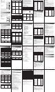
Example Operation Display
Temperature and length
of a steel bar
Temp Length
10ºC 1003mm
15ºC 1005mm
20ºC 1010mm
25ºC 1011mm
30ºC 1014mm
Using this table, the
regression formula and
correlation coefficient
can be obtained. Based
on the coefficient
formula, the length of
the steel bar at 18ºC
and the temperature
at 1000mm can be
estimated. Furthermore
the critical coefficient
(r
2
) and covariance can
also be calculated.
[
MODE
][3][1]
("REG" then select linear regression)
[
SHIFT
][Scl][=]
(Memory cleared)
10[
,
]1003[DT]
15[
,
]1005[DT]
20[
,
]1010[DT]
25[
,
]1011[DT]
30[
,
]1014[DT]
[
SHIFT
][A][=]
(Constant term A)
[
SHIFT
][B][=]
(Regression coefficient B)
[
SHIFT
][r][=]
(Correlation coefficient r)
18[
SHIFT
][y]
(Length at 18ºC)
1000
[
SHIFT
][x]
(Temp at 1
000
mm)
[
SHIFT
][r][x
2
][=]
(Critical coefficient)
[(][RCL][F][–][RCL][C][]
[
SHIFT
][
x
][][
SHIFT
][
y
][)][]
[(][
RCL
][
C
][
–
]1[)][=]
(Covariance)
0.
0.
10.
15.
20.
25.
30.
997.4
0.56
0.982607368
1007.48
4.642857143
0.965517241
35.
Example Operation Display
xi yi
29 1.6
50 23.5
74 38
103 46.4
118 48.9
The logarithmic
regression of the above
data, the regression
formula and correlation
coefficient are obtained.
Furthermore, respective
estimated values y and
x can be obtained for
xi = 80 and yi = 73 using
the regression formula.
[
MODE
][3][2]
("REG" then select LOG regression)
[
SHIFT
][Scl][=]
(Memory cleared)
29[
,
]1.6[DT]
50[
,
]23.5[DT]
74[
,
]38[DT]
103[
,
]46.4[DT]
118[
,
]48.9[DT]
[
SHIFT
][A][=]
(Constant term A)
[
SHIFT
][B][=]
(Regression coefficient B)
[
SHIFT
][r][=]
(Correlation coefficient r)
80[
SHIFT
][y]
(y when xi=80)
73
[
SHIFT
][x]
(x when yi=73)
0.
0.
29.
50.
74.
103.
118.
–111.1283975
34.02014748
0.994013946
37.94879482
224.1541314
Example Operation Display
xi yi
6.9 21.4
12.9 15.7
19.8 12.1
26.7 8.5
35.1 5.2
Through exponential
regression of the above
data, the regression
formula and correlation
coefficient are obtained.
Furthermore, the
regression formula is
used to obtain the
respective estimated
values of y and x, when
xi = 16 and yi = 20.
[
MODE
][3][3]
("REG" then select Exp regression)
[
SHIFT
][Scl][=]
(Memory cleared)
6.9[
,
]21.4[DT]
12.9[
,
]15.7[DT]
19.8[
,
]12.1[DT]
26.7[
,
]8.5[DT]
35.1[
,
]5.2[DT]
[
SHIFT
][A][=]
(Constant term A)
[
SHIFT
][B][=]
(Regression coefficient B)
[
SHIFT
][r][=]
(Correlation coefficient r)
16[
SHIFT
][y]
(y when xi=16)
20
[
SHIFT
][x]
(x when yi=20)
0.
0.
6.9
12.9
19.8
26.7
35.1
30.49758742
–0.049203708
–0.997247351
13.87915739
8.574868045
Example Operation Display
xi yi
28 2410
30 3033
33 3895
35 4491
38 5717
Through power
regression of the above
data, the regression
formula and correlation
coefficient are obtained.
Furthermore, the
regression formula is
used to obtain the
respective estimated
values of y and x, when
xi = 40 and yi = 1000.
[
MODE
][3][4][1]
("REG" then select Pwr regression)
[
SHIFT
][Scl][=]
(Memory cleared)
28[
,
]2410[DT]
30[
,
]3033[DT]
33[
,
]3895[DT]
35[
,
]4491[DT]
38[
,
]5717[DT]
[
SHIFT
][A][=]
(Constant term A)
[
SHIFT
][B][=]
(Regression coefficient B)
[
SHIFT
][r][=]
(Correlation coefficient r)
40[
SHIFT
][y]
(y when xi=40)
1000
[
SHIFT
][x]
(x when yi=1000)
0.
0.
28.
30.
33.
35.
38.
0.238801069
2.771866156
0.998906255
6587.674587
20.26225681