


Chapter 5 Root Locus Synthesis
Xmath Interactive Control Design Module 5-8 ni.com
Interpreting the Nonstandard Contour Plots
The Root Locus window can display phase contours other than the standard
180° as well as various magnitude contour plots. The meaning of these
curves is simple: if L(s)=a, then s would be a closed-loop pole if the loop
transfer function were multiplied by –1/a at the frequency s. For example,
a point s labeled ⏐L(s)⏐ = –3 dB on one of the 170° curves would be a
closed-loop pole if the loop transfer function at the frequency were to
increase in magnitude by 3 dB and increase in phase by 10°.
This simple observation works two ways. Continuing the previous
example, to have a pole at s, try to change the current controller to achieve
the required phase shift +10° and gain increase (+3 dB) at (for example,
by adding an appropriate pole-zero pair).
On the other hand, if the complex number is a poor place for a closed-loop
pole (for example, very lightly damped or unstable), then the current
compensator is not robust, since only a 10° phase shift along with 3 dB
of gain change in loop gain (most likely, the plant) would result in a
closed-loop pole at s. In this case, you turn to the problem of synthesizing
new compensation which decreases the phase and magnitude of the loop
transfer function at the frequency s. This has the effect of making the
closed-loop system less likely to have a pole at s when the plant transfer
function is changed; that is, it results in a more robust design.
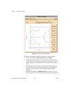
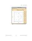
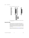
Figure 5-3 shows the Root Locus
window with the phase contours turned
off and the 0 dB magnitude contour turned on. The locus shows the set
of all possible closed-loop poles for the modified loop transfer function
L(s)=e
jθ
L(s) as θ varies from zero to 2π. By data-viewing the contour,
you can find the phase shift (value of θ) that corresponds to any point on
the locus.