


Chapter 2 Additive Error Reduction
Xmath Model Reduction Module 2-6 ni.com
with controllability and observability grammians given by,
in which the diagonal entries of Σ are in decreasing order, that is,
σ
1
≥σ
2
≥ ···, and such that the last diagonal entry of Σ
1
exceeds
the first diagonal entry of Σ
2
. It turns out that Reλ
i
( )<0 and
Reλ
i
(A
11
–A
12
A
21
)< 0, and a reduced order model G
r
(s) can be
defined by:
The attractive feature [LiA89] is that the same error bound holds as for
balanced truncation. For example,
Although the error bounds are the same, the actual frequency pattern of
the errors, and the actual maximum modulus, need not be the same for
reduction to the same order. One crucial difference is that balanced
truncation provides exact matching at ω = ∞, but does not match at DC,
while singular perturbation is exactly the other way round. Perfect
matching at DC can be a substantial advantage, especially if input signals
are known to be band-limited.
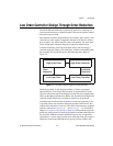
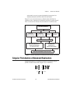
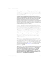
Singular perturbation can be achieved with
mreduce( ). Figure 2-1 shows
the two alternative approaches. For both continuous-time and discrete-time
reductions, the end result is a balanced realization.
Hankel Norm Approximation
In Hankel norm approximation, one relies on the fact that if one chooses an
approximation to exactly minimize one norm (the Hankel norm) then the
infinity norm will be approximately minimized. The Hankel norm is
defined in the following way. Let G(s) be a (rational) stable transfer
PQΣ
Σ
1
0
0 Σ
2
===
A
22
1–
A
22
1–
x
·
A
11
A
12
A
22
1–
A
21
–()xB
1
A
12
– A
22
1–
B
2
+()u+=
yC
1
C
2
A
22
1–
A
21
–()xDC
2
A
22
1–
B
2
–()u+=
Gjω()G
r
jω()–
∞
2trΣ
2
≤