


Chapter 4 Frequency-Weighted Error Reduction
Xmath Model Reduction Module 4-18 ni.com
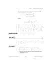
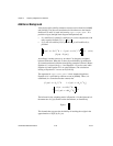
Controller reduction proceeds by implementing the same connection rule
but on reduced versions of the two transfer function matrices.
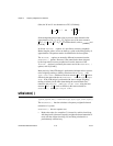
When K
E
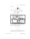
has been defined through Kalman filtering considerations, the
spectrum of the signal driving K
E
in Figure 4-5 is white, with intensity Q
yy
.
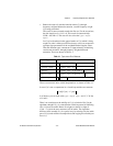
It follows that to reflect in the multiple input case the different intensities
on the different scalar inputs, it is advisable to introduce at some stage a
weight into the reduction process.
Algorithm
After preliminary checks, the algorithm steps are:
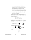
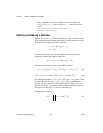
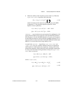
1. Form the observability and weighted (through Q
yy
) controllability
grammians of E(s) in Equation 4-7 by
(4-8)
(4-9)
2. Compute the square roots of the eigenvalues of PQ (Hankel singular
values of the fractional representation of Equation 4-5). The maximum
order permitted is the number of nonzero eigenvalues of PQ that are
larger than ε.
3. Introduce the order of the reduced-order controller, possibly by
displaying the Hankel singular values (HSVs) to the user. Broadly
speaking, one can throw away small HSVs but not large ones.
4. Using
redschur( )-type calculations, find a state-variable
description of E
r
(s). This means that E
r
(s) is the transfer function
matrix of a truncation of a balanced realization of E(s), but the
redschur( ) type calculations avoid the possibly numerically
difficult step of balancing the initially known realization of E(s).
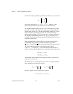
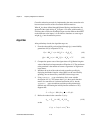
Suppose that:
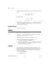
5. Define the reduced order controller C
r
(s) by
(4-10)
so that
Q
yy
12⁄
PA BK
R
–()′ABK
R
–()P+ K–
E
Q
yy
K
E
′
=
QA BK
R
–()ABK
R
–()′Q+ K
R
′
K
R
C′C––=
A
ˆ
S
lbig
′
ABK
R
–()S
rbig
K
E
, S
lbig
′
K
E
==
A
CR
S
lbig
′
ABK
R
– K
E
C–()S
rbig
=
C
r
s() C
CR
sI A
CR
–()
1–
B
CR
=