


Chapter 6 Tutorial
© National Instruments Corporation 6-3 Xmath Model Reduction Module
With a state weighting matrix,
Q = 1e-3*diag([2,2,80,80,8,8,3,3]);
R = 1;
(and unity control weighting), a state-feedback control-gain is determined
through a linear-quadratic performance index minimization as:
[Kr,ev] = regulator(sys,Q,R);
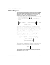
A – B × K
r
is stable. Next, with an input noise variance matrix Q = W
t
BBW
t
where,
and measurement noise covariance matrix =1, an estimation gain K
e
(so that A – K
e
C is stable) is determined:
Qhat = Wt*b*b'*Wt;
Rhat = 1;
[Ke,ev] = estimator(sys,Qhat,Rhat,{skipChks});
The keyword skipChks circumvents syntax checking in most functions.
It is used here because we know that
Qhat does not fulfill positive
semidefiniteness due to numerics).
sysc=lqgcomp(sys,Kr,Ke);
poles(sysc)
ans (a column vector) =
-0.296674 + 0.292246 j
-0.296674 - 0.292246 j
-0.15095 + 0.765357 j
-0.15095 - 0.765357 j
-0.239151 + 1.415 j
-0.239151 - 1.415 j
-0.129808 + 1.84093 j
-0.129808 - 1.84093 j
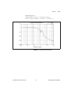
The compensator itself is open-loop stable. A brief explanation of how Q
and
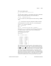
Wt are chosen is as follows. First, Q is chosen to ensure that the loop
gain (which would be relevant were the state measurable)
meets the constraints as far as possible. However, it is not possible to obtain
a 40 dB per decade roll-off at high frequencies, as LQ design virtually
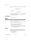
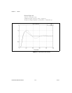
always yields a 20 dB per decade roll-off. Second, a loop transfer recovery
approach to the choice of as for some large ρ is modified through
the introduction of the diagonal matrix
Wt. The larger entries of Wt, because
of the modal coordinate system, in effect promote better loop transfer
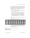
W
t
DIAG 0.346 0.346 0.024 0.0240.042 0.042, 0.042 0.042,,,,[]()=
R
ˆ
K
r
jωIA–()
1–
B
Q
ˆ
ρBB′