


Chapter 2 Additive Error Reduction
Xmath Model Reduction Module 2-14 ni.com
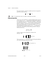
For the discrete-time case:
When
{bound} is specified, the error bound just enunciated is used to
choose the number of states in
SysR so that the bound is satisfied and nsr
is as small as possible. If the desired error bound is smaller than 2σ
ns
,
no reduction is made.
In the continuous-time case, the error depends on frequency, but is always
zero at ω = ∞. If the reduction in dimension is 1, or the system
Sys is
single-input, single-output, with alternating poles and zeros on the real
axis, the bound is tight. It is far from tight when the poles and zeros
approximately alternate along the jω-axis. It is not normally tight in the
discrete-time case, and for both continuous-time and discrete-time cases,
it is not tight if there are repeated singular values.
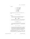
The presentation of the Hankel singular values may suggest a logical
dimension for the reduced order system; thus if , it may be
sensible to choose nsr = k.
Related Functions
ophank(), balmoore()
ophank( )
[SysR,SysU,HSV] = ophank(Sys,{nsr,onepass})
The ophank( ) function calculates an optimal Hankel norm reduction
of
Sys.
Restriction
This function has the following restriction:
• Only continuous systems are accepted; for discrete systems use
makecontinuous( ) before calling bst( ), then discretize the
result.
Sys=ophank(makecontinuous(SysD));
SysD=discretize(Sys);
Ge
jω
()G
R
e
jω
()–
∞
2 σ
nsr 1+
σ
nsr 2+
... σ
ns
+++()≤
σ
k
σ
k 1+
»