


Chapter 3 Multiplicative Error Reduction
© National Instruments Corporation 3-3 Xmath Model Reduction Module
bandwidth at the expense of being larger outside this bandwidth, which
would be preferable.
Second, the previously used multiplicative error is . In the
algorithms that follow, the error appears. It is easy to
check that:
and
This means that if either bound is small, so is the other, with the bounds
approximately equal.
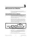
Two algorithms for multiplicative reduction are presented:
bst( ),
a mnemonic for balanced stochastic truncation, and
mulhank( ).
Roughly, they relate to one another in the same way that
redschur( )
and
ophank( ) relate, that is, one focuses on balanced realization
truncation and the other on Hankel norm approximation. Some of the
similarities and differences are as follows:
• When the errors are small, the error bound formula for
bst( ) is
about one half of that for
bst( ).
• With
bst( ), the actual multiplicative error as a function of frequency
goes to zero as ω→∞ (or, after using an optional transformation given
in the algorithm description, to zero as ω→ 0); with
mulhank( ), the
error tends to be more uniform as a function of frequency.
•
bst( ) can handle nonsquare reduction, while mulhank( ) cannot.
• Both algorithms are restricted to stable G(s); both preserve right half
plane zeros, that is, these zeros are copied into the reduced order
object; both have difficulties with jω-axis zeros of G(s), but these
difficulties are not insuperable.
bst( )
[SysR,HSV] = bst(Sys,{nsr,left,right,bound,method})
The bst( ) function calculates a balanced stochastic truncation of Sys for
the multiplicative case.
GG
ˆ
–()G
ˆ
1–
δ GG
ˆ
–()G
ˆ
1–
=
δ jω()
∞
∆ jω()
∞
1 ∆ jω()
∞
–
-------------------------------
≤
∆ jω()
∞
δ jω()
∞
1 δ jω()
∞
–
-------------------------------
≤