


Chapter 4 Frequency-Weighted Error Reduction
© National Instruments Corporation 4-5 Xmath Model Reduction Module
Fractional Representations
The treatment of jω-axis or right half plane poles in the above schemes is
crude: they are simply copied into the reduced order controller. A different
approach comes when one uses a so-called matrix fraction description
(MFD) to represent the controller, and controller reduction procedures
based on these representations (only for continuous-time) are found in
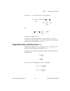
fracred( ). Consider first a scalar controller . One
can take a stable polynomial of the same degree as d, and then
represent the controller as a ratio of two stable transfer functions, namely
Now is the numerator, and the denominator. Write as
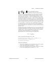
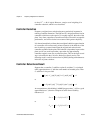
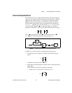
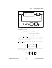
. Then we have the equivalence shown in Figure 4-1.
Figure 4-1. Controller Representation Through Stable Fractions
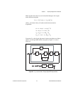
Evidently, C(s) can be formed by completing the following steps:
1. Construction of the one-input, two-output stable transfer function
matrix
(which has order equal to that of or ).
2. Interconnection through negative feedback of the second output to the
single input.
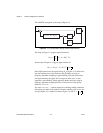
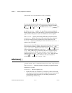
These observations motivate the reduction procedure:
• Reduce G to G
r
; notice that G is stable. Let G
r
be
Cs() ns()ds()⁄=
ds()
ns()
ds()
----------
ds()
ds()
----------
1–
nd⁄ dd⁄ dd⁄
1 ed⁄+
e
d
---
n
d
---
Cs()
G
nd⁄
ed⁄
=
d d
G
n
r
d
r
⁄
e
r
d
r
⁄
=