Chapter
7
Sampling Distributions
A large part of statistics consists of analyzing the probability of getting a sample mean or sample
proportion from a repeated number of samples drawn from the same population. Usually we
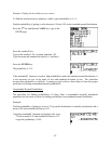
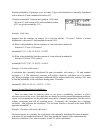
focus on two kinds of statistics from those samples: the sample mean Ë, if the data is
quantitative, or the sample proportion ê, if the data is categorical. For large sample sizes, both
Ë and ê have normal distributions which makes it much easier to compute their associated
probabilities. We will use the normalcdf( function on the calculator as described in Chapter 6
with a slight modification. As before, the answers using normalcdf( function will differ slightly
from the answers found from a table of normal probabilities, since the latter involves rounding.
Probabilities for Sample Means
For a large sample size, we know from the Central Limit Theorem that the sampling distribution
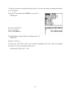
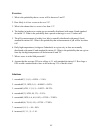
for the Ë is normally distributed with µ
Ë
= µ and σ
Ë
= σ/
n
.
To find the probability that a < Ë < b on the TI-83, TI-83 Plus, and TI-84 Plus calculators, use
normalcdf(a, b, µ, σ/
n
). The procedure is the same as finding the probability of a single value
except for the standard deviation being divided by the square root of the sample size. Remember
that if you are finding the area to the left of some value b, we use -1E99 for a. If you are finding
the area to the right of some value a, we use 1E99 for b.
Example: Cookie Weights
Assume that the weights of all packages of a certain brand of cookies are normally distributed
with a mean of 32 ounces and a standard deviation of 0.3 ounces. Find the probability that the
mean weight, Ë, of a random sample of 20 packages of this brand of cookies will be less than
31.8 ounces. The sample size here is not large, but the distribution is normal to begin with and
will remain normal as we average the measurements together.
46


