


Chapter 3 System Evaluation
MATRIXx Xmath Robust Control Module 3-2 ni.com
Refer to [BoB91] in Appendix A, Bibliography.
Example 3-1 Creating a Singular Value Plot
1. Let a system H be a 2-input/2-output system:
tf=makepoly([1,2],"s")/...
polynomial([0,-2.334,-12],"s")
tf (a transfer function) =
s + 2
--------------------
(s + 2.334)(s + 12)s
System is continuous
H = [tf, 2*tf; tf*tf, tf+3];
[outputs,inputs]=size(H)
outputs (a scalar) = 2
inputs (a scalar) = 2
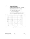
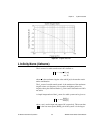
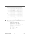
2. Now plot the singular values of the system between 0.01 and 100 Hz
using
svplot( ):
svplot(H,{Fmin=0.01,Fmax=100})
The result is shown in Figure 3-1. For a discussion of svplot( ) syntax,
refer to the Xmath Help.