


Chapter 4 Controller Synthesis
MATRIXx Xmath Robust Control Module 4-4 ni.com
The transfer matrix G can be viewed as a model of the underlying system
dynamics with v and u as generalized forces that produce effects in the
performance signals z and measured signals y.
The weight W
in
is used to model the exogenous input v by v = W
in
w.
Similarly, the critical performance variables in the vector z are weighted to
form the normal critical variables e = W
out
z.
In general, the input weight W
in
can be viewed as a dynamic model of the
exogenous inputs and the output weight W
out
as the inverse of the desired
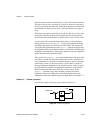
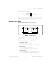
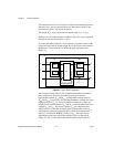
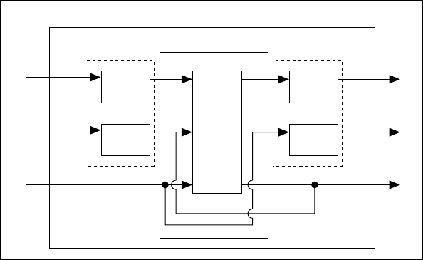
performance. As an illustration, consider the plant configuration in
Figure 4-3.
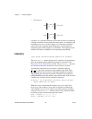
Figure 4-3. Typical Plant Configuration
The exogenous input vectors d and n represent disturbances and sensor
noise, respectively. These are generated by passing normalized
unpredictable signals, ω
dist
and ω
noise
, through stable transfer matrices,
W
dist
and W
noise
, respectively. The critical performance variables are some
regulated variables y
reg
, as well as the actuator commands u. These are
weighed by the transfer matrices W
reg
and W
act
to form the normalized error
variables e
reg
and e
act
. The sensed variables y
sens
are contaminated by
additive noise n to form the measured signal y. The transfer matrix G
dyn
represents the underlying system dynamics. Observe that the transfer
matrix G, as defined in [BBK88], consists of G
dyn
with some special
output/input connections among the variables n and u as depicted in
Figure 4-3. This is in the form of the familiar LQG setup, except that
w
d
n
y
reg
y
sens
u
e
u
y
P
W
dist
w
dist
W
in
W
reg
W
out
w
e
W
noise
w
noise
e
reg
e
act
W
act
G
dyn
G