


Chapter 3 System Evaluation
© National Instruments Corporation 3-5 MATRIXx Xmath Robust Control Module
•If A has an imaginary eigenvalue at jω
0
, linfnorm( ) returns:
vOMEGA =
SIGMA = Infinity
where ω
0
is one of the imaginary eigenvalues of A.
•Even if H is unstable,
linfnorm( ) returns its maximum singular
value on the jω axis.
For discrete-time systems
linfnorm( ) converts a discrete-time L
∞
norm computation problem to a continuous-time problem using a Cayley
transformation. For example, it maps the unit circle conformally onto the
complex right half plane using a linear fractional transformation. The
linfnorm( ) function then calls itself to solve the continuous-time
problem, and finally converts the solution back to discrete-time.
Example 3-2 Example of linfnorm( )
Sys=system([-0.2,-1;1,0],[1,0]',[0,1],0);
[sigma,omega]=linfnorm(Sys)
sigma (a scalar) = 5.07322
omega (a scalar) = 0.157081
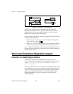
The linfnorm( ) function will return the L
∞
norm (sigma) of the transfer
matrix H(jω) described by
Sys, and omega is the vector of frequencies
where it is achieved.
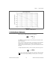
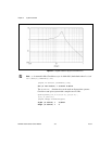
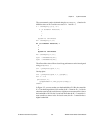
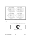
linfnorm( ) computation can be checked by
plotting the singular values of H(jω) as a function of ω (Figure 3-2).
sv=svplot(Sys,{fmin=.01, fmax=1.0});
ω
0