


More about Integration D–5
File name 32sii-Manual-E-0424
Printed Date : 2003/4/24 Size : 17.7 x 25.2 cm
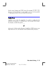
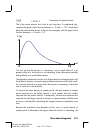
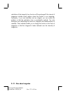
f (x)
x
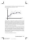
The graph is a spike very close to the origin. Because no sample point
happened to discover the spike, the algorithm assumed that f(x) was
identically equal to zero throughout the interval of integration. Even if you
increased the number of sample points by calculating the integral in SCI 11
or ALL format, none of the additional sample points would discover the spike
when this particular function is integrated over this particular interval. (For
better approaches to problems such as this, see the next topic, "Conditions
That Prolong Calculation Time.")
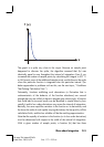
Fortunately, functions exhibiting such aberrations (a fluctuation that is
uncharacteristic of the behavior of the function elsewhere) are unusual
enough that you are unlikely to have to integrate one unknowingly. A function
that could lead to incorrect results can be identified in simple terms by how
rapidly it and its low–order derivatives vary across the interval of integration.
Basically, the more rapid the variation in the function or its derivatives, and
the lower the order of such rapidly varying derivatives, the less quickly will the
calculation finish, and the less reliable will be the resulting approximation.
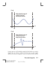
Note that the rapidity of variation in the function (or its low–order derivatives)
must be determined with respect to the width of the interval of integration.
With a given number of sample points, a function f(x) that has three