


572 Appendix B: Reference Information
8992APPB DOC TI
-
89/TI
-
92 Plus:8992a
pp
b doc (English) SusanGullord Revised:02/23/01 1:54 PM Printed: 02/23/01 2:24 PM Page 572 of 34
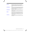
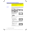
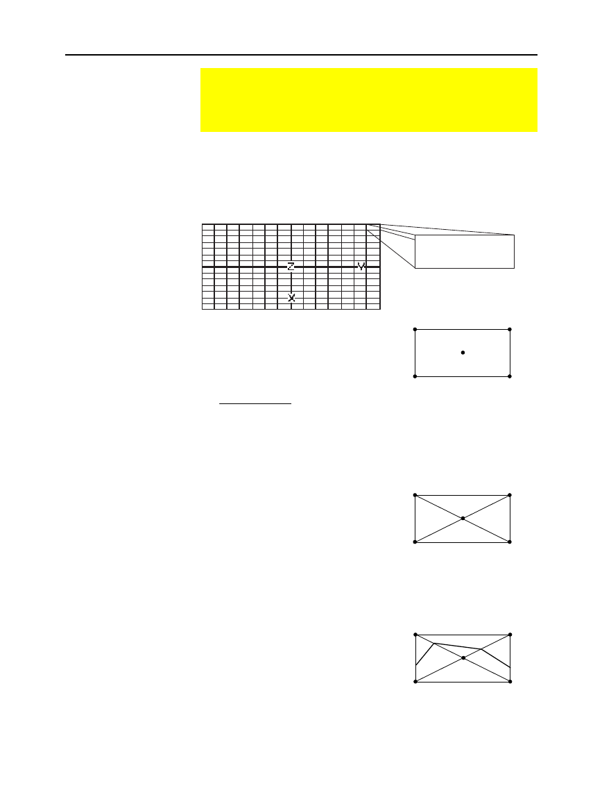
Based on your
x
and
y
Window variables, the distance between
xmin
and
xmax
and between
ymin
and
ymax
is divided into a number of grid
lines specified by
xgrid
and
ygrid
. These grid lines intersect to form a
series of rectangles.
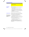
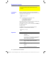
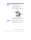
For each rectangle, the equation is
evaluated at each of the four
corners (also called vertices or
grid points) and an average value
(
E
) is calculated:
E =
z
1
+ z
2
+ z
3
+ z
4
4
The
E
value is treated as the value of the equation at the center of the
rectangle.
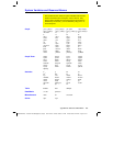
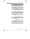
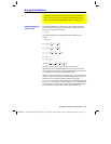
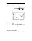
For each specified contour value
(
C
i
):
¦ At each of the five points
shown to the right, the
difference between the point’s
z
value and the contour value
is calculated.
¦ A sign change between any two adjacent points implies that a
contour crosses the line that joins those two points. Linear
interpolation is used to approximate where the zero crosses the
line.
¦ Within the rectangle, any zero
crossings are connected with
straight lines.
¦ This process is repeated for
each contour value.
Each rectangle in the grid is treated similarly.
Contour Levels and Implicit Plot Algorithm
Contours are calculated and plotted by the following method.
An implicit plot is the same as a contour, except that an implicit
plot is for the z=0 contour only.
Algorithm
z
1
=f(x
1
,y
1
)
z
3
=f(x
2
,y
1
)
E
z
2
=f(x
1
,y
2
)
z
4
=f(x
2
,y
2
)
z
1
ìC
i
z
3
ìC
i
EìC
i
z
2
ìC
i
z
4
ìC
i