5-36
Math Menu
re-entered, the View Parameters function will re-display the best fit curve
and the parameter window.
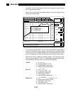
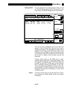
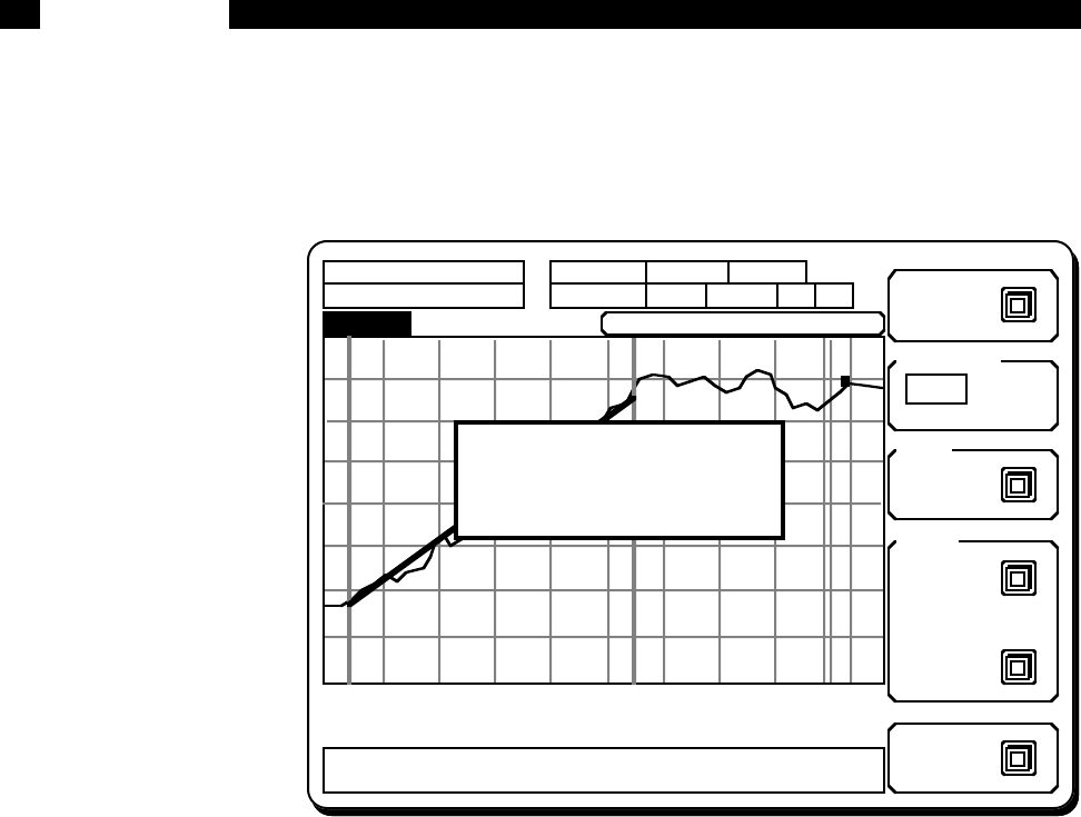
Both the Do Fit and View Parameters functions result in a display screen
like the one shown below.
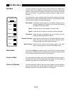
In this example screen, the fit is a line. The curve fit region is delimited by
the two limit markers (heavy dashed vertical lines) as described below.
The final curve fit is plotted between the limit markers along with the
data. The parameters of the fit are displayed in the window at the center.
Each type of fit has a different parameter display. The horizontal coordi-
nate is t (cursor readout in time, i.e. increasing to the right) and the verti-
cal coordinate is the trace value (in the units of the display).
Line Fit:
y = a + b•(t - t
0
)
t
0
= horizontal offset in time
a = vertical offset in trace units
b = slope in trace units/second
Exp. Fit:
y = ae
-(t - t
0
)/b
+ c
t
0
= horizontal offset in time
a = amplitude in trace units
b = time constant in time
c = vertical offset in trace units
Gauss. Fit:
y = ae
-
1/2
(∆t/b)
2
+ c where ∆t = t - t
0
t
0
= peak center position in time
a = amplitude in trace units
b = line width in time
c = vertical offset in trace units
center = 0.0
±
50.00 e-3 V
10 S /div
Y 7.000 S 36.100 e-3
0.000 S
y = a + b•(t-t0)
t0 = 9.600000e+001 s
a = -2.875882e-003
b = 1.136381e-003
Press Any Key To Continue...
Full Scale = 100 mV
Dyn Reserve = 23 dB
100 mS
12 dB/oct Line 2xLin AC A
Syncro
Line
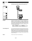
Type of Fit
View
Limits
Exp
Gauss
Do Fit:
Params:
Left:
Right:
Return:


