


20060301
14-7-7
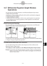
Differential Equation Graph Window Operations
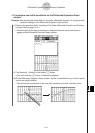
(3) From the eActivity application menu, tap [Insert], [Strip], and then [DiffEqGraph].
• This inserts a Differential Equation Graph data strip,
and displays the Differential Equation Graph window
in the lower half of the screen.
S
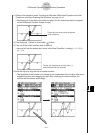
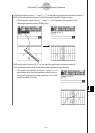
To graph the slope field and solution curves by dropping a 1st-order
differential equation and matrix into the Differential Equation Graph
window
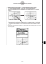
Example: To drag the 1st-order differential equation
y
’
= exp(
x
) +
x
2
and then the initial
condition matrix [0,1] from the eActivity application window to the Differential
Equation Graph window, and graph the applicable slope field and solution curve
(1) On the application menu, tap
.
• This starts up the eActivity application.
(2) On the eActivity application window, input the following expression and matrix.
y
’
= exp(
x
) +
x
2
[0,1]
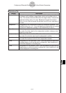
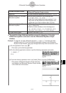
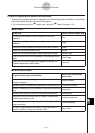
To draw this type of graph:
Drop this type of expression or value into the
Differential Equation Graph window:
Slope field 1st-order differential equation in the form of
y'
=
f
(
x
,
y
)
Solution curve(s) of a 1st-order
differential equation
Matrix of initial conditions in the following form:
[[
x
1
,
y
(
x
1
)][
x
2
,
y
(
x
2
)], .... [
x
n
,
y
(
x
n
)]]
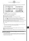
• Slope field must already have been graphed. If not,
only points will be plotted and initial conditions are
registered in the initial condition editor ([IC] tab).
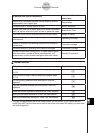
Solution curve(s) of an Nth-order
differential equation
1) Nth-order differential equation such as
y’’
+
y’
+
y
=
sin(
x
), followed by
2) Matrix of initial conditions in the following form:
[[
x
1
,
y
1(
x
1
)],[
x
2
,
y
1(
x
2
)], .... [
x
n
,
y
1(
x
n
)]] or [[
x
1
,
y
1(
x
1
),
y
2(
x
1
)],[
x
2
,
y
1(
x
2
),
y
2(
x
2
)], .... [
x
n
,
y
1(
x
n
),
y
2(
x
n
)]]
f
(
x
) type function graph Function in the form
y
=
f
(
x
)