144 CHAPTER 4. DEMONSTRATION EXAMPLES
g2 = starp(himat
ic,k2)
comment g2 "closed loop: iteration 2"
[,,nx] = size(k2)
display "k2 now also has " + string(nx) + " states"
k2 now also has 20 states
This design probably resulted in a control law which achieved an infinity norm of
approximately 1.1 for the new interconnection structure.
k2 has been designed to reduce µ(g2). The singular values may actually get worse. We
will see that this is the case here.
The stability of g2 is examined with the function check. As used here, it will return a 1
if it is stable and a zero if not. A frequency response is then calculated.
check(g2,{stable})
ans (a scalar) = 1
g2g=freq(g2,om2)
comment g2g "g2 frequency response"
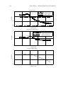
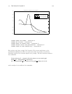
The µ analysis is repeated to assess the closed loop robust performance of the µ based
controller (k2). The command format is identical to the last time.
[bnds2,D2,D2inv,Delta2,sens2] = mu(g2g,blk)
gph6 = ctrlplot(bnds2,{log,line
style=[1,4]});
gph6 = ctrlplot(bnds1,gph6,{log,line
style=[3,5]});
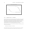
gph6 = plot(gph6,{title="Robustness analysis for the g2 system",...
legend=["g2: mu upper bound";"g2: mu lower bound";...
"g1: mu upper bound";"g1: mu lower bound"],!grid})?


