2.4. µ ANALYSIS 49
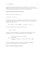
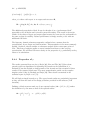
Actually, the lower bound is always equal to µ but the implied optimization has local
maxima which are not global. For the upper bound Safonov and Doyle [72], have shown
that finding the infimum is a convex problem and hence more easily solved. However the
bound is equal to µ only in certain special cases. Here we use the infimum rather that
the miminum because D may have a element which goes to zero as the maximum
singular value decreases. So the limiting case (where an element of D is zero) is not a
member of the set D.
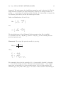
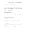
The cases where the upper bound is equal to µ are tabulated below.
q =0 q=1 q=2
m=0 equal less than or equal
m =1 equal equal less than or equal
m =2 equal less than or equal less than or equal
m =3 equal less than or equal less than or equal
m =4 less than or equal less than or equal less than or equal
Most practical applications of the µ theory involve models where q = 0. Here we see that
we have equality with the upper bound for three or fewer blocks. Computational
experience has yet to produce an example where the bound differs by more than
15 percent. In practically motivated problems the gap is usually much less.
2.4.5 The Main Loop Theorem
We will introduce a fundamental theorem in µ analysis: the main loop theorem. From
the previous discussion you will see that there are several matrix properties that can be
expressed as µ tests. The spectral radius and the maximum singular value are two such
quantities. The main loop theorem gives a way of testing such properties for perturbed
systems. The test is simply a larger µ problem. This is the theorem underlying the
extension from robust stability to robust performance.
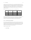
Consider a partitioned matrix,
M =
M
11
M
12
M
21
M
22
,


