2.4. µ ANALYSIS 51
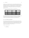
2.4.6 State-space Robustness Analysis Tests
We will look at some more advanced state-space approaches to the analysis of robust
performance. Most users of the software will concentrate on the more common frequency
domain analysis methods covered in Section 2.4.3. The analysis tests given here can be
implemented with the Xµ functions and the more advanced user can use these to study
the robustness of systems with respect to time-varying and nonlinear perturbations.
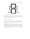
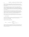
To illustrate this approach, consider the state-space LFT model of a system introduced
in Section 2.2.4. A digital system is described by,
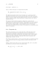
x(k +1) = Ax(k)+Bu(k)
y(k)=Cx(k)+Du(k).
This digital system has transfer function,
P(z)=F
u
(P
ss
,z
−1
I),
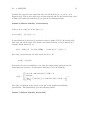
where P
ss
is the real valued matrix,
P
ss
=
AB
CD
,
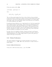
and the scalar × identity, z
−1
I, has dimension nx, equal to the state dimension of P(z).
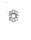
This is now in the form of an LFT model with a single scalar × identity element in the
upper loop.
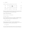
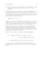
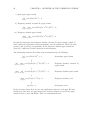
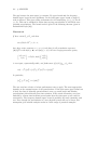
Define,
∆
1
=
δI
nx
δ ∈C
,
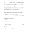
and note that with this definition,
µ
1
(A)=ρ(A).


