24 CHAPTER 2. OVERVIEW OF THE UNDERLYING THEORY
systems. We will now look at other possible perturbation structures. For more detail on
these structures (in the complex case) refer to Packard and Doyle [20].
Consider a blocks which are of the form scalar × identity, where the scalar is unknown.
In the following we will include q of these blocks in ∆. The definition of ∆ is therefore
modified to be,
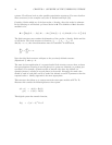
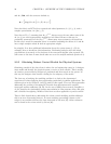
∆ =
diag(δ
1
I
1
,...,δ
q
I
q
,∆
1
,...,∆
m
)
dim(I
j
)=l
j
×l
j
,dim(∆
i
)=k
i
×k
i
.(2.9)
The block structure now contains the dimension of the q scalar × identity blocks and the
m full blocks. The block structure is therefore, (l
1
,...,l
q
,k
1
,...,k
m
). If
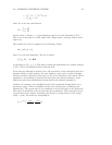
dim(∆) = n × n, then these dimensions must be consistent. In otherwords,
q
j=1
l
j
+
m
i=1
k
i
= n.
Note that this block structure collapses to the previously defined structure
(Equation 2.7) when q =0.
The most obvious application of a repeated scalar block structure occurs when we know
that perturbations occurring in several places in a system are identical (or perhaps just
correlated). For example, dynamic models of aircraft often have the altitude (or
dynamic pressure) occuring in several places in the model. Naturally the same value
should be used in each place and if we model the altitude as an LFT parameter then the
repeated scalar × identity approach is the most appropriate.
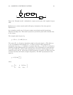
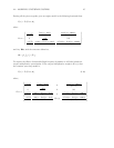
This structure also allows us to express uncertain state-space models as LFTs. To
illustrate this consider the following discrete time system.
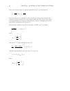
x(k +1) = Ax(k)+Bu(k)
y(k)=Cx(k)+Du(k).
This digital system has transfer function,
P(z)=C(zI − A)
−1
B + D


