


SECTION 7. MEASUREMENT PROGRAMMING EXAMPLES
7-12
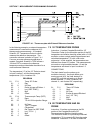
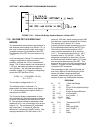
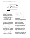
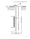
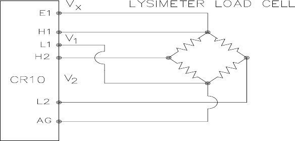
FIGURE 7.13-2. 6 Wire Full Bridge Connection for Load Cell
copper changes 0.4% per degree C change in
temperature. Assume that the cable between the
load cell and the CR10 lays on the soil surface
and undergoes a 25°C diurnal temperature
fluctuation. If the resistance is 33 ohms at the
maximum temperature, then at the minimum
temperature, the resistance is:
(1-25x0.004)33 ohms = 29.7 ohms
The actual excitation voltage at the load cell is:
V
1
= 350/(350+29.7) V
x
= .92 V
x
The excitation voltage has increased by 1%,
relative to the voltage applied at the CR10. In the
case where we were recording a 91 mm change
in water content, there would be a 1 mm diurnal
change in the recorded water content that would
actually be due to the change in temperature.
Instruction 9 solves this problem by actually
measuring the voltage drop across the load cell
bridge. The drawbacks to using Instruction 9 are
that it requires an extra differential channel and
the added expense of a 6 wire cable. In this
case, the benefits are worth the expense.
The load cell has a nominal full scale output of 3
millivolts per volt excitation. If the excitation is 2.5
volts, the full scale output is 7.5 millivolts; thus, the
±7.5 millivolt range is selected. The calibrated
output of the load cell is 3.106 mV/V
1
at a load of
250 pounds. Output is desired in millimeters of
water with respect to a fixed point. The "4" found
in equation 7.13-1 is due to the mechanical
advantage. The calibration in mV/V
1
/mm is:
3.106 mV/V
1
/250 lb x 2.2 lb/kg x
3.1416 kg/mm/4 = 0.02147 mV/V
1
/mm
The reciprocal of this gives the multiplier to
convert mV/V
1
into millimeters. (The result of
Instruction 9 is the ratio of the output voltage to
the actual excitation voltage multiplied by 1000,
which is mV/V
1
):
1/0.02147 mV/V
1
/mm = 46.583 mm/mV/V
1
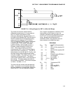
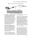
The output from the load cell is connected so
that the voltage increases as the mass of the
lysimeter increases. (If the actual mechanical
linkage was as shown in Figure 7.13-1, the
output voltage would be positive when the load
cell was under tension.)
When the experiment is started, the water content
of the soil in the lysimeter is approximately 25% on
a volume basis. It is decided to use this as the
reference (i.e., 0.25 x 1500 mm = 375 mm). The
experiment is started at the beginning of what is
expected to be a period during which
evapotranspiration exceeds precipitation.
Instruction 9 is programmed with the correct
multiplier and no offset. After hooking everything
up, the counterbalance is adjusted so that the load
cell is near the top of its range; this will allow a
longer period before readjustment is necessary.
The result of Instruction 9 (monitored with the *6
Mode) is 109. The offset needed to give the
desired initial value of 375 mm is 266. However, it
is decided to add this offset in a separate
instruction so the result of Instruction 9 can be
used as a ready reminder of the strain on the load
cell (range = ±140 mm). When the strain on the
load cell nears its rated limits, the counterbalance
is readjusted and the offset recalculated to provide
a continuous record of the water budget.
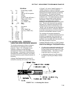
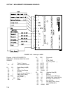
The program table has an execution interval of 10
seconds. The average value in millimeters is output
to Final Storage (not shown in Table) every hour.