


3-20
Making Time Domain Measurements
Time Domain Low Pass Mode
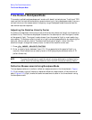
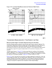
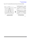
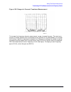
Figure 3-15 Time Domain Low Pass Measurement of an Amplifier Small Signal
Transient Response
Interpreting the Low Pass Step Transmission Response Horizontal Axis
The low pass transmission measurement horizontal axis displays the average transit time
through the test device over the frequency range used in the measurement. The response
of the thru connection used in the calibration is a step that reaches 50% unit height at
approximately time = 0. The rise time is determined by the highest frequency used in the
frequency domain measurement. The step is a unit high step, which indicates no loss for
the thru calibration. When a device is inserted, the time axis indicates the propagation
delay or electrical length of the device. The markers read the electrical delay in both time
and distance. The distance can be scaled by an appropriate velocity factor as described in
"Time Domain Bandpass Mode" on page 3-12.
Interpreting the Low Pass Step Transmission Response Vertical Axis
In the real format, the vertical axis displays the transmission response in real units (for
example, volts). For the amplifier example in Figure 3-15, if the amplifier input is a step of
1 volt, the output, 2.4 nanoseconds after the step (indicated by marker 1), is 5.84 volts.
In the log magnitude format, the amplifier gain is the steady state value displayed after
the initial transients die out.
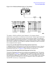
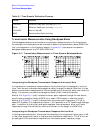
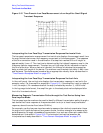
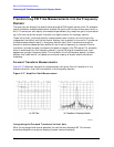
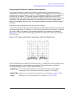
Measuring Separate Transmission Paths through the Test Device Using Low
Pass Impulse Mode
The low pass impulse mode can be used to identify different transmission paths through a
test device that has a response at frequencies down to dc (or at least has a predictable
response, above the noise floor, below 50 MHz).
For example, use the low pass impulse mode to measure the relative transmission times
through a multi-path device such as a power divider. Another example is to measure the
pulse dispersion through a broadband transmission line, such as a fiber optic cable. Both
examples are illustrated in Figure 3-16. The horizontal and vertical axes can be
interpreted as already described in "Time Domain Bandpass Mode" on page 3-12.