


252
Example 16
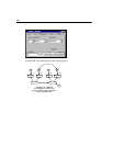
Most of these parameter estimates are not very interesting, although you may want to
check and make sure that the estimates are reasonable. We have already noted that the
variance estimates are positive. The path coefficients in the measurement model are
positive, which is reassuring. A mixture of positive and negative regression weights in
the measurement model would have been difficult to interpret and would have cast
doubt on the model. The covariance between eps2 and eps4 is positive in both groups,
as expected.
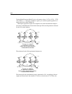
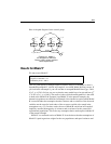
We are primarily interested in the regression of post_verbal on pre_verbal. The
intercept, which is fixed at 0 in the control group, is estimated to be 3.71 in the
experimental group. The regression weight is estimated at 0.95 in the control group and
0.85 in the experimental group. The regression weights for the two groups are close
enough that they might even be identical in the two populations. Identical regression
weights would allow a greatly simplified evaluation of the treatment by limiting the
comparison of the two groups to a comparison of their intercepts. It is therefore
worthwhile to try a model in which the regression weights are the same for both
groups. This will be Model D.
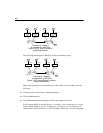
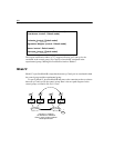
Model D
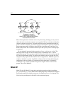
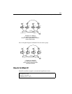
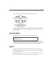
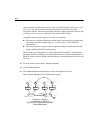
Model D is just like Model C except that it requires the regression weight for predicting
post_verbal from pre_verbal to be the same for both groups. This constraint can be imposed
by giving the regression weight the same name, for example pre2post, in both groups. The
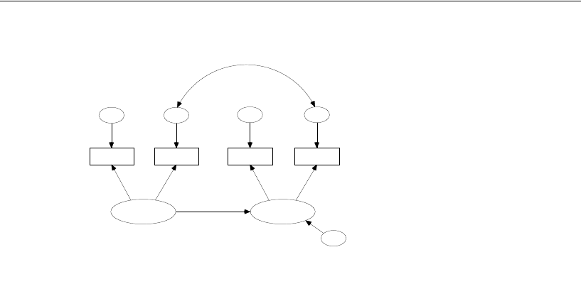
following is the path diagram for Model D for the experimental group:
1.87, 47.46
pre_verbal
18.63
pre_syn
0, 2.19
eps1
1.00
1
19.91
pre_opp
0, 12.39
eps2
.88
1
3.71
post_verbal
20.38
post_syn
0, 7.51
eps3
21.21
post_opp
0, 17.07
eps4
1.00
1
.90
1
.85
0, 8.86
zeta
1
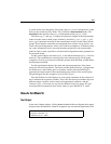
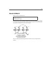
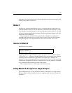
Example 16: Model C
An alternative to ANCOVA
Olsson (1973): experimental condition.
Unstandardized estimates
7.34