403
Bayesian Estimation
E
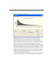
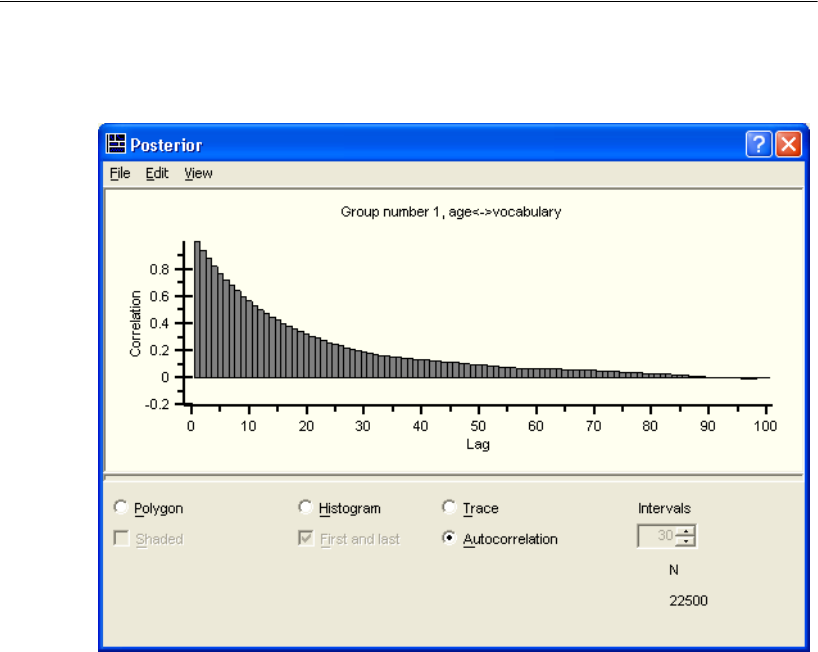
To display this plot, select Autocorrelation.
Lag, along the horizontal axis, refers to the spacing at which the correlation is
estimated. In ordinary situations, we expect the autocorrelation coefficients to die
down and become close to 0, and remain near 0, beyond a certain lag. In the
autocorrelation plot shown above, the lag-10 correlation—the correlation between any
sampled value and the value drawn 10 iterations later—is approximately 0.50. The
lag-35 correlation lies below 0.20, and at lag 90 and beyond, the correlation is
effectively 0. This indicates that by 90 iterations, the MCMC procedure has essentially
forgotten its starting position, at least as far as this covariance parameter is concerned.
Forgetting the starting position is equivalent to convergence in distribution. If we were
to examine the autocorrelation plots for the other parameters in the model, we would
find that they also effectively die down to 0 by 90 or so iterations. This fact gives us
confidence that a burn-in period of 500 samples was more than enough to ensure that
convergence in distribution was attained, and that the analysis samples are indeed
samples from the true posterior distribution.
In certain pathological situations, the MCMC procedure may converge very slowly
or not at all. This may happen in data sets with high proportions of missing values,


