260
Example 16
covariances of the exogenous variables) imply the assumptions of Model X (equal
covariances for the observed variables). Models X and Y are therefore nested models,
and it is possible to carry out a conditional test of Model Y under the assumption that
Model X is true. Of course, it will make sense to do that test only if Model X really is
true, and we have already concluded it is not. Nevertheless, let’s go through the
motions of testing Model Y against Model X. The difference in chi-square values is
2.671 (that is, 31.816 – 29.145) with 2 (= 12 – 10) degrees of freedom. These figures
are identical (within rounding error) to those of Example 9, Model B. The difference
is that in Example 9 we assumed that the test was appropriate. Now we are quite sure
(because we rejected Model X) that it is not.
If you have any doubts that the current Model Y is the same as Model B of Example
9, you should compare the parameter estimates from the two analyses. Here are the
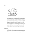
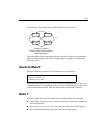
Model Y parameter estimates for the 108 experimental subjects. See if you can match
up these estimates displayed with the unstandardized parameter estimates obtained in
Model B of Example 9.
Model Z
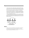
Finally, construct a new model (Model Z) by starting with Model Y and adding the
requirement that the intercept in the equation for predicting post_verbal from
pre_verbal be the same in both populations. This model is equivalent to Model C of
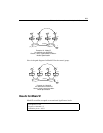
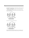
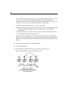
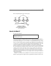
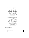
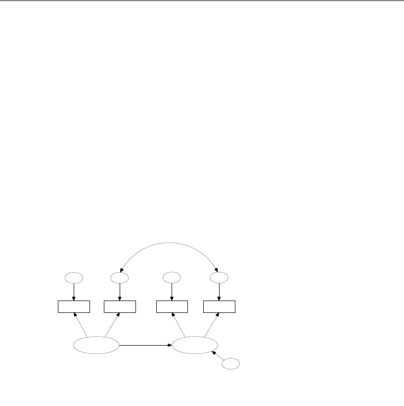
Example 9. The path diagrams for Model Z are as follows:
1.88, 37.79
pre_verbal
18.53
pre_syn
0, 6.04
eps1
1.00
1
19.90
pre_opp
0, 12.31
eps2
.88
1
3.64
post_verbal
20.38
post_syn
0, 6.58
eps3
21.20
post_opp
0, 14.75
eps4
1.00
1
.91
1
.89
0, 4.85
zeta
1
Example 16: Model Y
An alternative to ANCOVA
Olsson (1973): experimental condition.
Unstandardized estimates
6.83


