


616
Appendix C
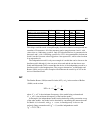
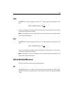
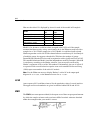
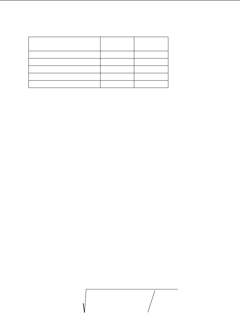
Here are the critical N’s displayed by Amos for each of the models in Example 6:
Model A, for instance, would have been accepted at the 0.05 level if the sample
moments had been exactly as they were found to be in the Wheaton study but with a
sample size of 164. With a sample size of 165, Model A would have been rejected.
Hoelter argues that a critical N of 200 or better indicates a satisfactory fit. In an analysis
of multiple groups, he suggests a threshold of 200 times the number of groups.
Presumably this threshold is to be used in conjunction with a significance level of 0.05.
This standard eliminates Model A and the independence model in Example 6. Model B
is satisfactory according to the Hoelter criterion. I am not myself convinced by
Hoelter’s arguments in favor of the 200 standard. Unfortunately, the use of critical N
as a practical aid to model selection requires some such standard. Bollen and Liang
(1988) report some studies of the critical N statistic.
Note: Use the \hfive text macro to display Hoelter’s critical N in the output path
diagram for , or the \hone text macro for .
LO 90
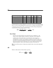
Amos reports a 90% confidence interval for the population value of several statistics.
The upper and lower boundaries are given in columns labeled HI 90 and LO 90.
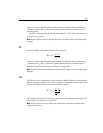
RMR
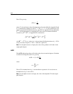
The RMR (root mean square residual) is the square root of the average squared amount
by which the sample variances and covariances differ from their estimates obtained
under the assumption that your model is correct.
Model
HOELTER
0.05
HOELTER
0.01
Model A: No Autocorrelation 164 219
Model B: Most General 1615 2201
Model C: Time-Invariance 1925 2494
Model D: A and C Combined 216 277
Independence model 11 14
α 0.05=
α 0.01=
()
()
∑∑∑∑
===
≤
=
⎪
⎭
⎪
⎬
⎫
⎪
⎩
⎪
⎨
⎧
−=
G
g
g
G
g
p
i
ij
j
g
ij
g
ij
ps
g
1111
)()(
*
ˆ
RMR
σ