259
Sörbom’s Alternative to Analysis of Covariance
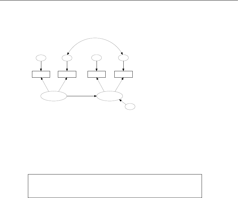
Here is the path diagram for the control group:
Results for Model Y
We must reject Model Y.
This is a good reason for being dissatisfied with the analysis of Example 9, since it
depended upon Model Y (which, in Example 9, was called Model B) being correct. If
you look back at Example 9, you will see that we accepted Model B there (χ
2
= 2.684,
df = 2, p = 0.261). So how can we say that the same model has to be rejected here (χ
2
= 31.816, df = 1, p = 0.001)? The answer is that, while the null hypothesis is the same
in both cases (Model B in Example 9 and Model Y in the present example), the
alternative hypotheses are different. In Example 9, the alternative against which Model
B is tested includes the assumption that the variances and covariances of the observed
variables are the same for both values of the treatment variable (also stated in the
assumptions on p. 35). In other words, the test of Model B carried out in Example 9
implicitly assumed homogeneity of variances and covariances for the control and
experimental populations. This is the very assumption that is made explicit in Model X
of the present example.
Model Y is a restricted version of Model X. It can be shown that the assumptions of
Model Y (equal regression weights for the two populations, and equal variances and
Chi-square = 31.816
Degrees of freedom = 12
Probability level = 0.001
0, v_v1
pre_verbal
a_syn1
pre_syn
0, v_e1
eps1
1
1
a_opp1
pre_opp
0, v_e2
eps2
opp_v1
1
0
post_verbal
a_syn2
post_syn
0, v_e3
eps3
a_opp2
post_opp
0, v_e4
eps4
1
1
opp_v2
1
pre2post
0, v_z
zeta
1
Example 16: Model Y
An alternative to ANCOVA
Olsson (1973): control condition.
Model S
ecification
