


401
Bayesian Estimation
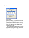
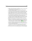
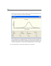
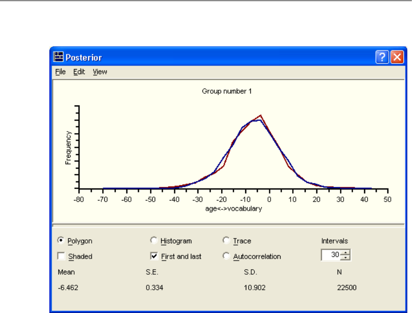
In this example, the distributions of the first and last thirds of the analysis samples are
almost identical, which suggests that Amos has successfully identified the important
features of the posterior distribution of the age-vocabulary covariance. Note that this
posterior distribution appears to be centered at some value near –6, which agrees with
the Mean value for this parameter. Visual inspection suggests that the standard
deviation is roughly 10, which agrees with the value of S.D.
Notice that more than half of the sampled values are to the left of 0. This provides
mild evidence that the true value of the covariance parameter is negative, but this result
is not statistically significant because the proportion to the right of 0 is still quite large.
If the proportion of sampled values to the right of 0 were very small—for example, less
than 5%—then we would be able to reject the null hypothesis that the covariance
parameter is greater than or equal to 0. In this case, however, we cannot.
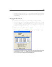
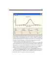
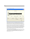
Another plot that helps in assessing convergence is the trace plot. The trace plot,
sometimes called a time-series plot, shows the sampled values of a parameter over
time. This plot helps you to judge how quickly the MCMC procedure converges in
distribution—that is, how quickly it forgets its starting values.