479
Censored Data
To fit the model:
E Click on the toolbar.
or
E From the menus, choose Analyze > Bayesian Estimation.
Note: The button is disabled because, with non-numeric data, you can perform only
Bayesian estimation.
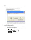
After the Bayesian SEM window opens, wait until the unhappy face changes into
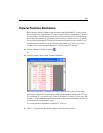
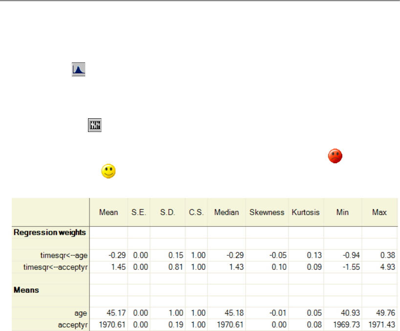
a happy face . The table of estimates in the Bayesian SEM window should look
something like this:
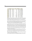
(Only a portion of the table is shown in the figure.) The
Mean column contains point
estimates for the parameters. The regression weight for using acceptyr to predict
timesqr is 1.45, so that each time the calendar advances by one year, you predict an
increase of 1.45 in the square root of survival time. This suggests that the transplant
program may have been improving over the period covered by the study. The
regression weight for using age to predict timesqr is –0.29, so for every year older a
patient is when admitted into the transplant program, you expect a decrease of 0.29 in
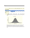
the square root of survival time. The regression weight estimate of –0.29 is actually the
mean of the posterior distribution of the regression weight.
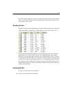
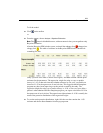
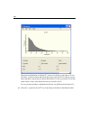
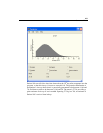
E To see the entire posterior distribution, right-click the row that contains the –0.29
estimate and choose
Show Posterior from the pop-up menu.


