


172 Chapter 10: 3D Graphing
10_3D.DOC TI-89/TI-92 Plus: 3D Graphing (English) Susan Gullord Revised: 02/23/01 11:00 AM Printed: 02/23/01 4:22 PM Page 172 of 2210_3D.DOC TI-89/TI-92 Plus: 3D Graphing (English) Susan Gullord Revised: 02/23/01 11:00 AM Printed: 02/23/01 4:22 PM Page 172 of 22
¦
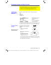
The viewing angle is set initially so that you are viewing the plot
by looking down the z axis. You can change the viewing angle as
necessary.
¦
The plot is shown in expanded view. To switch between
expanded and normal view, press
p
.
¦
The
Labels
format is set to
OFF
automatically.
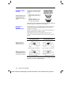
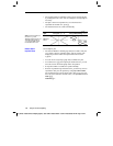
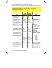
Style
xñìyñ =4
z1(x,y)=xñìyñì4
sin(x)+cos(y)=
e
(x
ù
y)
z1(x,y)=sin(x)+cos(y)ì
e
(x
ù
y)
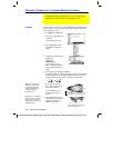
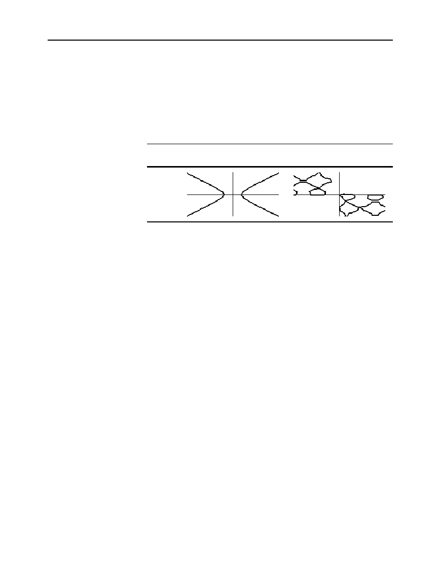
IMPLICIT
PLOT
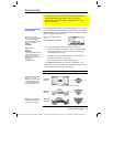
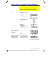
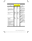
For an implicit plot:
¦ The
ncontour
Window variable (page 168) has no affect. Only the
z=0 contour is drawn, regardless of the value of
ncontour
. The
displayed plot shows where the implicit form intersects the
xy plane.
¦ You can use the cursor keys (page 164) to animate the plot.
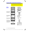
¦ You cannot trace (
…
) the implicit plot itself. However, you can
trace the unseen wire frame graph of the 3D equation.
¦ It may take awhile to evaluate the equation initially.
¦ Because of possible long evaluation times, you first may want to
experiment with your 3D equation by using
Style=WIRE FRAME
.
The evaluation time is much shorter. Then, after you’re sure you
have the correct Window variable values, set
Style=IMPLICIT PLOT
.
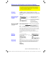
TI
-
89:
¥Í
TI
-
92 Plus
:
¥
F
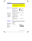
Note: These examples use
the same
x
,
y
, and
z
Window variable values as
a
ZoomStd viewing cube. If
y
ou use ZoomStd, press
Z
to look down the z axis.
Notes About
Implicit Plots