


178 Chapter 11: Differential Equation Graphing
11DIFFEQ.DOC TI-89/TI-92 Plus: Differential Equation (English) Susan Gullord Revised: 02/23/01 11:04 AM Printed: 02/23/01 2:15 PM Page 178 of 26
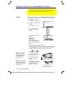
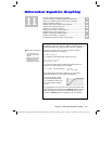
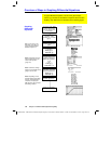
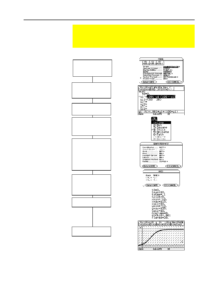
Overview of Steps in Graphing Differential Equations
To graph differential equations, use the same general steps
used for y(x) functions as described in Chapter 6: Basic Function
Graphing. Any differences are described on the following pages.
Graphing
Differential
Equations
Set Graph mode (3)
to
DIFF EQUATIONS
.
Also set Angle mode,
if necessary.
Define equations and,
optionally, initial
conditions on Y= Editor
(¥ #).
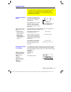
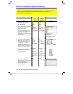
Select (†) which
defined equations to
graph.
Set the display style for
an equation.
TI
-
89
: 2
ˆ
TI
-
92 Plus:
ˆ
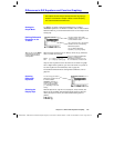
Define the viewing
window (¥ $).
Set the graph format.
Solution Method and
Fields are unique to
differential equations.
ƒ
9
— or —
TI
-
89:
¥
Í
TI
-
92 Plus:
¥
F
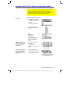
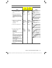
Set the axes as
applicable, depending
on the Fields format.
TI
-
89:
2
‰
TI
-
92 Plus:
‰
Note:
The
Fields
format is
critical, depending on the
order of the equation
(page 197).
Note:
Depending on the
Solution Method
and
Fields
formats, different Window
variables are displayed.
Tip:
„ Zoom
also changes
the viewing window.
Note:
Valid
Axes
settings
depend on the
Fields
format
(pages 190 and 197).
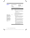
Graph the equations
(¥ %).
Tip:
To turn off any stat
data plots, press
‡ 5
or
use
†
to deselect them.
Refer to Chapter 16.