


Chapter 11: Differential Equation Graphing 191
11DIFFEQ.DOC TI-89/TI-92 Plus: Differential Equation (English) Susan Gullord Revised: 02/23/01 11:04 AM Printed: 02/23/01 2:15 PM Page 191 of 26
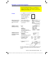
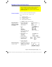
Use the two coupled 1st-order differential equations:
y1' =
ë
y1 + 0.1y1
ù
y2
and
y2' = 3y2
ì
y1
ù
y2
where:
y1
= Population of foxes
yi1
= Initial population of foxes (2)
y2
= Population of rabbits
yi2
= Initial population of rabbits (5)
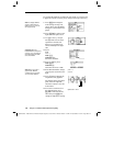
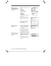
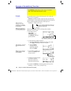
1. Use
3
to set
Graph
=
DIFF EQUATIONS
.
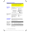
2. In the Y= Editor (
¥#
),
define the differential
equations and enter the
initial conditions.
3. Press:
ƒ
9
— or —
TI
-
89:
¥
Í
TI
-
92 Plus:
¥
F
Set
Axes = ON
,
Labels = ON
,
Solution Method = RK
, and
Fields
=
FLDOFF
.
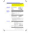
4. In the Y= Editor, press:
TI
-
89
:
2‰
TI
-
92 Plus:
‰
Set
Axes = TIME
.
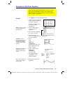
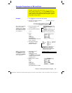
5. In the Window Editor
(
¥$
), set the
Window variables.
t0=0. xmin=
ë
1. ncurves=0.
tmax=10. xmax=10. diftol=.001
tstep=
p
/24 xscl=5.
tplot=0. ymin=
ë
10.
ymax=40.
yscl=5.
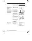
6. Graph the differential
equations (
¥%
).
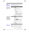
7. Press
…
to trace. Then press
3
¸
to see the number of
foxes (
yc
for
y1
) and rabbits
(
yc
for
y2
) at
t=3
.
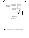
Example of Time and Custom Axes
Using the predator-prey model from biology, determine the
numbers of rabbits and foxes that maintain population
equilibrium in a certain region. Graph the solution using both
time and custom axes.
Predator-Prey Model
Tip: To speed up graphing
times, clear any other
equations in the Y= Editor.
With
FLDOFF
, all equations
are evaluated even if they
are not selected.
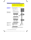
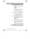
Tip: Use
C
and
D
to move
the trace cursor between th
e
curves for y1 and y2.
y1(t)
y2(t)