


Chapter 11: Differential Equation Graphing 175
11DIFFEQ.DOC TI-89/TI-92 Plus: Differential Equation (English) Susan Gullord Revised: 02/23/01 11:04 AM Printed: 02/23/01 2:15 PM Page 175 of 26
Chapter 11:
Differential Equation Graphing
Preview of Differential Equation Graphing........................................ 176
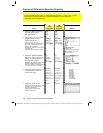
Overview of Steps in Graphing Differential Equations..................... 178
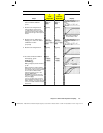
Differences in Diff Equations and Function Graphing...................... 179
Setting the Initial Conditions................................................................ 184
Defining a System for Higher-Order Equations ................................. 186
Example of a 2nd-Order Equation ....................................................... 187
Example of a 3rd-Order Equation........................................................ 189
Setting Axes for Time or Custom Plots............................................... 190
Example of Time and Custom Axes .................................................... 191
Example Comparison of RK and Euler ............................................... 193
Example of the deSolve( ) Function.................................................... 196
Troubleshooting with the Fields Graph Format ................................ 197
This chapter describes how to solve differential equations
graphically on the
TI
-
89 / TI
-
92 Plus
. Before using this chapter, you
should be familiar with Chapter 6: Basic Function Graphing.
The
TI
-
89 / TI
-
92 Plus
solves 1st-order systems of ordinary
differential equations. For example:
y' = .001 y
ù
(100
ì
y)
or coupled 1st-order differential equations such as:
y1' =
ë
y1 + 0.1
ù
y1
ù
y2
y2' = 3
ù
y2
ì
y1
ù
y2
You can solve higher-order equations by defining them as a
system of 1st-order equations. For example:
y'' + y = sin(t)
can be defined as
y1' = y2
y2' =
ë
y1 + sin(t)
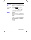
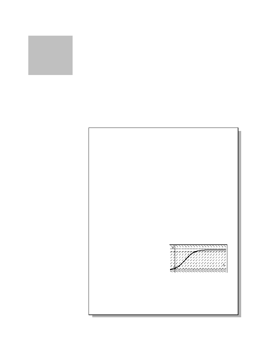
By setting appropriate initial conditions, you can graph a
particular solution curve of a differential equation.
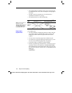
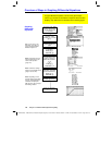
You can also graph a slope
or direction field that helps
you visualize the behavior of
the entire family of solution
curves.
For graphing, the
TI
-
89 / TI
-
92 Plus
uses numerical methods that
approximate the true solutions. The
deSolve()
function lets you
solve some differential equations symbolically. This chapter
introduces
deSolve()
. Refer to Appendix A for more details.
11
Note: A differential equation
is:
• 1st-order
when only
1st-order derivatives
appear.
•
Ordinary
when all the
derivatives are with
respect to the same
independent variable.