


570 Appendix B: Reference Information
8992APPB DOC TI
-
89/TI
-
92 Plus:8992a
pp
b doc (English) SusanGullord Revised:02/23/01 1:54 PM Printed: 02/23/01 2:24 PM Page 570 of 34
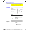
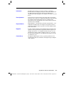
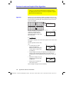
Most of the regressions use non-linear recursive least-squares
techniques to optimize the following cost function, which is the sum
of the squares of the residual errors:
[]
J residualExpression
i
N
=
=
∑
1
2
where:
residualExpression
is in terms of
x
i
and
y
i
x
i
is the independent variable list
y
i
is the dependent variable list
N
is the dimension of the lists
This technique attempts to recursively estimate the constants in the
model expression to make
J
as small as possible.
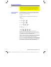
For example,
y=a sin(bx+c)+d
is the model equation for
SinReg
. So
its residual expression is:
a sin(bx
i
+c)+d
ì
y
i
For
SinReg
, therefore, the least-squares algorithm finds the
constants
a
,
b
,
c
, and
d
that minimize the function:
[]
Jabxcdy
ii
i
N
=++−
=
∑
sin
()
2
1
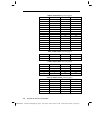
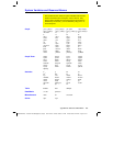
Regression Description
CubicReg
Uses the least-squares algorithm to fit the third-order
polynomial:
y
=
ax
3
+
bx
2
+
cx
+
d
For four data points, the equation is a polynomial fit;
for five or more, it is a polynomial regression. At
least four data points are required.
ExpReg
Uses the least-squares algorithm and transformed
values
x
and ln(
y
) to fit the model equation:
y
=
ab
x
LinReg
Uses the least-squares algorithm to fit the model
equation:
y
=
ax
+
b
where
a
is the slope and
b
is the y-intercept.
Regression Formulas
This section describes how the statistical regressions are
calculated.
Least-Squares
Algorithm
Regressions