Page 10-13
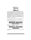
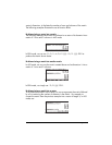
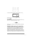
In RPN mode, with the 3×3 matrix in the stack, we simply have to activate
function DI G to obtain the same result as above.
Function DIAG→
Function DIAG→ takes a vector and a list of matrix dimensions {rows, columns},
and creates a diagonal matrix with the main diagonal replaced with the proper
vector elements. For example, the command
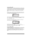
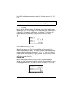
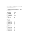
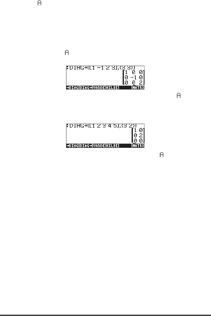
DI G([1,-1,2,3],{3,3})
produces a diagonal matrix with the first 3 elements of the vector argument:
In RPN mode, we can use [1,-1,2,3] ` {3,3}` DI G to
obtain the same result as above.
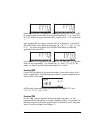
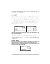
Another example of application of the DIAG
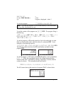
→ function follows, in ALG mode:
In RPN mode, use [1,2,3,4,5] ` {3,2}` DI G .
In this case a 3×2 matrix was to be created using as main diagonal elements as
many elements as possible form the vector [1,2,3,4,5]. The main diagonal, for
a rectangular matrix, starts at position (1,1) and moves on to position (2,2),
(3,3), etc. until either the number of rows or columns is exhausted. In this case,
the number of columns (2) was exhausted before the number of rows (3), so the
main diagonal included only the elements in positions (1,1) and (2,2). Thus,
only the first two elements of the vector were required to form the main
diagonal.
Function VANDERMONDE
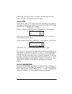
Function VANDERMONDE generates the Vandermonde matrix of dimension n
based on a given list of input data. The dimension n is, of course, the length of
the list. If the input list consists of objects {x
1
, x
2
,… x
n
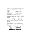
}, then, a Vandermonde
matrix in the calculator is a matrix made of the following elements:


