


Page 16-12
Example 3 – Determine the inverse Laplace transform of F(s) = sin(s). Use:
‘SIN(X)’ ` ILAP. The calculator takes a few seconds to return the result:
‘ILAP(SIN(X))’, meaning that there is no closed-form expression f(t), such that f(t)
= L
-1
{sin(s)}.
Example 4
– Determine the inverse Laplace transform of F(s) = 1/s
3
. Use:
‘1/X^3’ ` ILAP μ. The calculator returns the result: ‘X^2/2’, which is
interpreted as L
-1
{1/s
3
} = t
2
/2.
Example 5
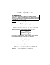
– Determine the Laplace transform of the function f(t) = cos (a⋅t+b).
Use: ‘COS(a*X+b)’ ` LAP . The calculator returns the result:
Press μ to obtain –(a sin(b) – X cos(b))/(X
2
+a
2
). The transform is interpreted
as follows: L {cos(a⋅t+b)} = (s⋅cos b – a⋅sin b)/(s
2
+a
2
).
Laplace transform theorems
To help you determine the Laplace transform of functions you can use a number
of theorems, some of which are listed below. A few examples of the theorem
applications are also included.
Θ Differentiation theorem for the first derivative
. Let f
o
be the initial condition
for f(t), i.e., f(0) = f
o
, then
L{df/dt} = s⋅F(s) - f
o
.
Θ Differentiation theorem for the second derivative
. Let f
o
= f(0), and (df/dt)
o
= df/dt|
t=0
, then L{d
2
f/dt
2
} = s
2
⋅F(s) - s⋅f
o
– (df/dt)
o
.
Example 1
– The velocity of a moving particle v(t) is defined as v(t) = dr/dt,
where r = r(t) is the position of the particle. Let r
o
= r(0), and R(s) =L{r(t)}, then,
the transform of the velocity can be written as V(s) = L{v(t)}=L{dr/dt}= s⋅R(s)-r
o
.