


Page 22-17
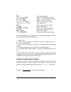
@)PPAR Show plot parameters
{ θ 0 6.29} ` @INDEP Define ‘θ’ as the indep. Variable
~y` @DEPND Define ‘Y’ as the dependent variable
3 \# 3 @XRNG Define (-3,3) as the x-range
0.5 \# 2.5 @YRNG L Define (-0.5,2.5) as the y-range
{ (0,0) {.5 .5} “x” “y”} ` Axes definition list
@AXES Define axes center, ticks, labels
L @)PLOT Return to PLOT menu
@ERASE @DRAX L @LABEL Erase picture, draw axes, labels
L @DRAW Draw function and show picture
@)EDIT L@MENU Remove menu labels
LL@)PICT @CANCL Return to normal calculator display
From these examples we see a pattern for the interactive generation of a two-
dimensional graph through the PLOT menu:
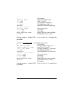
1 – Select PTYPE.
2 – Store function to plot in variable EQ (using the proper format, e.g.,
‘X(t)+iY(t)’ for PARAMETRIC).
3 – Enter name (and range, if necessary) of independent and dependent
variables
4 – Enter axes specifications as a list { center atick x-label y-label }
5 – Use ERASE, DRAX, LABEL, DRAW to produce a fully labeled graph with
axes
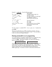
This same approach can be used to produce plots with a program, except that
in a program you need to add the command PICTURE after the DRAW function
is called to recall the graphics screen to the stack.
Examples of program-generated plots
In this section we show how to implement with programs the generation of the
last three examples. Activate the PLOT menu before you start typing the
program to facilitate entering graphing commands („ÌC, see above).
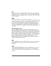
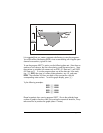
Example 1 – A function plot
. Enter the following program: