Page 16-69
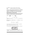
contain only the value of ε, and the step Δx will be taken as a small default
value. After running function @@RKF@@, the stack will show the lines:
2: {‘x’, ‘y’, ‘f(x,y)’ ‘∂f/∂x’ ‘∂f/vy’ }
1: { εΔx }
The value of the solution, y
final
, will be available in variable @@@y@@@.
This function can be used to solve so-called “stiff” differential equations.
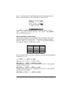
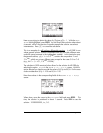
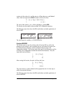
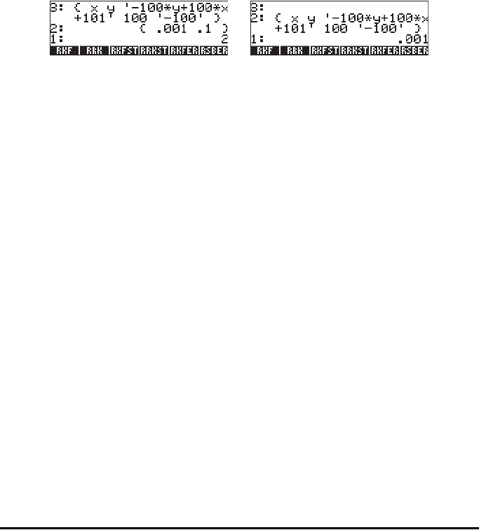
The following screen shots show the RPN stack before and after application of
function RRK:
The value stored in variable y is 3.00000000004.
Function RKFSTEP
This function uses an input list similar to that of function RKF, as well as the
tolerance for the solution, and a possible step Δx, and returns the same input
list, followed by the tolerance, and an estimate of the next step in the
independent variable. The function returns the input list, the tolerance, and the
next step in the independent variable that satisfies that tolerance. Thus, the
input stack looks as follows:
ˆˍʳʳʳʳʳʳ {‘x’, ‘y’, ‘f(x,y)’}
2: ε
1: Δx
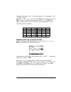
After running this function, the stack will show the lines:
3: {‘x’, ‘y’, ‘f(x,y)’}
2: ε
1: (Δx)
next
Thus, this function is used to determine the appropriate size of a time step to
satisfy the required tolerance.
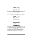
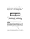
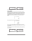
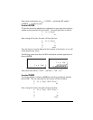
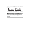
The following screen shots show the RPN stack before and after application of
function RKFSTEP:


